Write a MATLAB program to perform Otto cycle And plot PV diagram.

AIM = Write a MATLAB program to plotting PV diagram for air standard cycle

OBJECTIVES

1. plotting PV diagram for otto cycle.
2. Determining the air standard efficiency (therma lefficiency).

THEORY

Air Standard Cycle: The cycle in which air is usedas aworking substance is called anair standard cycle

Air standard efficiency:Ratio of work done by the system to heat input to the system is known as an "Air Standard Efficiency". This efficiency is ideal efficiency.

Thermal efficiency = work done / heat supplied.

Air standard assumptions:

1. The working fluid is air, Which continuosly circumstances in a closed and always behaves as an ideal gas.
2. All the processes that make that make up the cycle are internally reversible.
3. The combustion process is replaced by a heat-addition process from an enternal source.
4. The exhaust process is replaced by a heat-rejection process that restores the working fluid to its initial state.
5. The physical constants of air are constant.

THE OTTO CYCLE :

An otto cycle is idealised thermodynamic cycle that describesthe functioning of a typical spark ignition piston engine. It is the thermodynamic cycle most commonly found in automobile engines.

Otto cycle is a description of what happens to gas it is subjected to changes of volume, temperature, addition, or removal of heat. The processes involved during this cycle are as follows.

1. Process 1-2: Isentropic compression
2. Process 2-3: Constant volume and heat addition
3. Process 3-4: Isentropic expansion
4. Process 4-1: Constant volume heat reject

1. Process 1-2: Adiabatic compression of the charge as the piston moves from the bottom dead centre (BDC) to top dead centre(TDC).

2. Process 2-3: Constant-volume heat transfer to the working gas from an external source while the piston is at top dead centre. This process is intended to represent the ignition of the fuel-air mixture and the subsequent rapid burning.

3. Process 3-4: Adiabatic expansion (Power stoke)

4. Process 4-1: Completes the cycle by a constant-volume process in which heat is rejected from the air while the piston is at bottom dead centre.

PISTON KINEMATICS

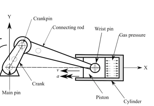
Input parametres:

Cylinder Bore Length(b) = 0.1 metres

Stroke Length (s) = 0.1 metres

Connecting Rod-length = 0.15 metres

Compression Ratio of the engine (cr) = 12

Pressure at 1st state (p1) = 1 atm (101325 pa)

Temperature at 1st state(t1) = 500k

Temperature at 3rd state (t3) = 2300k

Ratio of cp and cv (gamma) = 1.4 (from air and diatomic gases)

The Kinematics equations pertinent to this project:

volume swept (v_s) = (pi/4).bore^2.stoke

volume clearance (v_c) = v_s/(cr-1)

Volume at the 1st state (v1) = v_s + v_c

Volume at the 2nd state (v2) = v_c

1. Write a MATLAB program to plotting Pv diagram for air standard cycle.

clear all
close all
clc

%inputs
gamma = 1.4;
t3 = 2300;
%state variables 1
p1 = 101325;
t1 = 500;

%engine geometric variables
bore = 0.1;
stroke = 0.1;
con_rod = 0.15;
cr = 12;

%calculating the swept volume and the clearance volume 
v_swept = (pi/4)*bore^2*stroke;
v_clearance = v_swept/(cr-1);

v1 = v_swept+v_clearance;
v2 = v_clearance;

%state variables of state point 2
%p2*v2^gamma = p1*v1^gamma | p2 = p1*cr^gamma 
p2 = p1*(cr)^gamma;

%p1*v1/t1 = p2*v2/t2 |t2 = p2*v2*t1/p1*v1
t2 = ((p2*v2)*t1)/(p1*v1);

constant_c = p1*v1^gamma;
 V_compression = engine_kinematics(bore, stroke, con_rod, cr, 180, 0);
 P_compression = constant_c./V_compression.^gamma;

%state variables of state point 3
v3 = v2
%p3*v3/t3 = p2*v2/t2 | p3 = p2*(t3/t2)
p3 = p2*(t3/t2);

constant_c = p3*v3^gamma;
 V_expansion = engine_kinematics(bore, stroke, con_rod, cr, 0, 180);
 P_expansion = constant_c./V_expansion.^gamma;

%state variables at state point 4
v4 = v1
%p3*v3^gamma = p4*v4^gamma | p4 = p3*(v3/v4)^gamma
p4 = p3*((v3/v4)^gamma);

%p3*v3/t3 = p4*v4/t4 | t4 = ((p4*v4)*t3)/(p3*v3)
t4 = ((p4*v1)*t3)/(p3*v3);

%thermal efficiency
thermal_efficiency = 1-((t4-t1)/(t3-t2))

figure(1)
hold on
plot(v1,p1,'*','Color','r')
plot(V_compression,P_compression)
plot(v2,p2,'*','Color','r')
plot([v2,v3],[p2,p3])
plot(V_expansion,P_expansion)
plot(v3,p3,'*','Color','r')
plot(v4,p4,'*','Color','r')
plot([v4,v1],[p4,p1])
xlabel('volume')
ylabel('pressure')

function [V] = engine_kinematics(bore,stroke,con_rod,cr,starting_crank,ending_crank);

a = stroke/2;
R = con_rod/a;


v_s = pi/4*bore^2*stroke;
v_c = v_s/(cr-1);

theta = linspace(starting_crank,ending_crank,100);

term1 = 0.5*(cr-1);
term2 = R+1-cosd(theta);
term3 = (R^2 - sind(theta).^2).^0.5;

V = (1 + term1*(term2 - term3)).*v_c;
end

EXPLAIN THE PROGRAM

To write a program that would give the output as the PV diagram of the otto cycle and the overall thermal efficiency of the cycle.

So we need some inputs to start the program, here the constants inputs is

gamma(`gamma`) = 1.4 and Temperature t3 = 2300k

now we had to define the state variables(these variables represent a particular condition)

p1 = 101325 pa i.e atmospheric pressure and t1 = 500k

After that now we get the geometric parametres of engine. Basic parametres is

bore = 0.1,stroke = 01, connecting rod length = 0.15,compression ratio(cr)= 12. Using these parametres we obtain clearance volume, swept volume, V1 and V2 i.e volume at state point 1 and 2.

now calculate state variables at state point 2 we will use the following relation `p2*(v2)^gamma=p1*(v1)^gamma`. Using this relation we get the value of p2. for calculating t2 we use this following relation

`frac(p1*v1 )(t1) = frac(p2*v2) (t2)|`

So for compression volume (Vcompression) we will use the following formula:

`V/(Vc) = 1+1/2(cr-1)[R+1-costheta-(R^2-sin^2theta)^(1/2)]`

Vc is clearance volume

cr is compression ratio

`theta`is the crank angle

R is the ratio of connecting rod length/crank pin radius

Here i have used the function command and created a function known as engine_kinemtics(). it will gives an ease of passing different values for the input parametres of the function.

In the function engine_kinematics i used the above formula and broke it down in different terms to better simplify it. For getting `theta`i have used linspace command to get the angles from start of the crank to the end of the crank rotation. So the `theta`that we take is from `180^circ to 0^circ`as it compressing so the volume is reducing. so we obtain Vcompression.

`t the state variable at point 3 us this relation `frac(p3*v3)(t3) = frac(p2*v2)(t2)``to get state variables p3.

v3=v2 as it is an process where no volume is change .

also along the isentropic process there is constsnt p1*(v1)^gamma= constant/(Vcompression)^gamma

Same process is applied for expansion process Vexpansion the `theta`will be `o^circ to 180^circ` we will use the same relation

p3*(v3)^gamma = constant

Pexpansion = constant/(Vexpansion)^gamma

To find the state variables at point 4 we use the relation `p3*(v3)^gamma = p4*(v4)^gamma` we get p4 using `frac(p3*v3)(t3) = frac(p4*v4)(t4)` we find theb value of t4.

For the Thermal efficiency we use this formula:

`etathermal = 1-frac(t4-t1)(t3-t2)`

At the values of t1 t2 t3 t4 wwere obtained from above relations, this help us finding nthe thermal efficiency of the cycle is 62.99% or 0.6299.

For the plot of the PV diagram I used the different values of pressure(p1,p2,Pcompression,p3,Pexpansion) volume (v1,v2,Vcompression,v3,Vexpansion, v4)

OUTPUT:

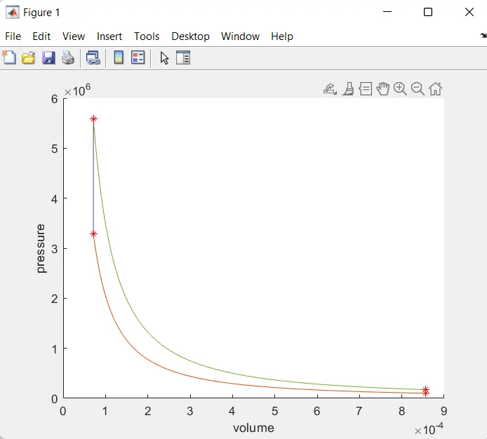
PV diagram:

Thermal efficiency of the cycle:

ERROR#1: To plot PV diagram

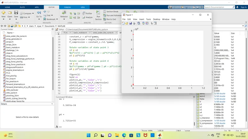
SOLUTION#: To plot PV diagram

in #Line48: plot(Vcompression, P_compression) is written then it occured error

actual program is plot(P_compression, V_compression) is right.

RESULTS & CONCLUSION:

1. The PV diagram of Otto cycle has been plotted successfully.

2. The air standard efficiency(`eta`thermal) was found to be 62.99%.

3. Hence,air standard efficieny depends only bon compression ratio.

4. for High compression ratio, air standard efficiency is high.

5. But at higher compression ratios knocking occurs, hence an optimum compression ratio must be selected.