Week 4.1 - Genetic Algorithm

AIM: To optimize the stalagmite function and find the global maximaof the function using MATLAB code.

OBJECTIVE: To explain the concept of genetic algorithm and it's syntax and also to find the global maxima of the function.

DESCRIPTION:

GENETIC ALGORITHMS:

God is the creator of the whole universe. Ever since its creation evolution has been a part and parcel of its functioning. New organisms have envolved from their ancestors; and this evolution is governed by a simple law which charles darwin as - "survival of the fittest".

Genetic algorithms are search alorithms based on natural selection amd natural genetics. They combine survival of fittest among structureswith structured yet randomized information exchange to form a search alogritm.

Genetic algorithms(GA) provide a general approch for dearching for global minima or maxima within a bounded, quantized search space.

As a result, it is hard to classify a "generic" or "traditional" GA, since there are so many variants. However, by studying the original ideas involved with the early GA and studying other variants.

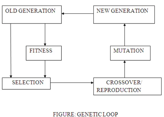
Five phases are considered in a gentic algorithms

1. Initial population
2. Fitness function
3. Selection
4. Crossover
5. Mutation

Initial population: The set of individuals involved in the process is called as population. Each individual is a solution to the problem you want to solve.

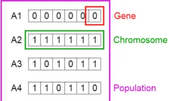
Fitness function: The function in which determines how fit an individual is to complete with others.

Selection: The phase of selecting the more fittest individual. individuals with high fitness have more chance to getting to be selected.

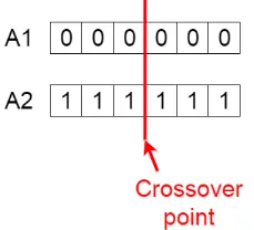
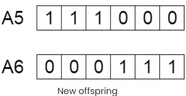
Cross Over: It is the most significant phase in a genetic algorithm. For each pair of parenta to be mated, a crossover point is chosen at random from within the genes.

For example, consider the crossover to be 3 as shown below

Offspring are created by exchanging the genes of parents among themselves until the crossover point is reached.

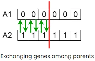
The new offspring are added to the population.

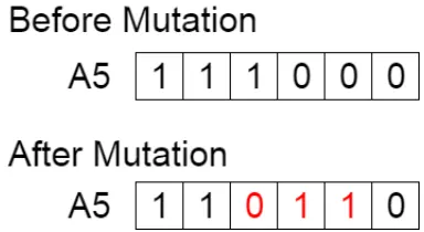
Mutation: Mutation occurs to maintain diversity within the population and prevent premature convergence.

OPTIMIZATION:

Optimization is the area of study which deals with how to minimize or maximize a particular function which depends upon multiple input parametres. It involves the selection of best element from the available set of alternatives.

Local maximas refers to tiny peaks. The objective of the optimization is to determine the global maxima without having prior knowledge of the other peaks.

STALAGMITE FUNCTION:

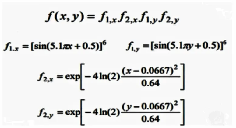
Stalagmite function is the mathematical model that acutually helps us to gain local maximas and minimas. A stalagmite is the type of rock formation that rises from the floor of the cave due to the accumulation of materials deposited on the floor from ceiling drippings. Stalagmite may be composed of lava, minerals,sand etc.

Stalagmite can be plotted as a function ehich is defined as:

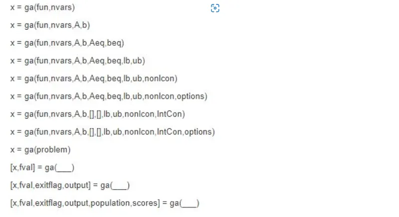
GA SYNTAX:

The genetic algorithms uses three main types of rules at each step to create the next generation from the current population.

• Selection rules select the individuals,called parents, that contibute to the population at the next generation.
• Crossover rules combine two parents to form children for the next generation.
• Mutation rules apply random changes to individual parents to form children.

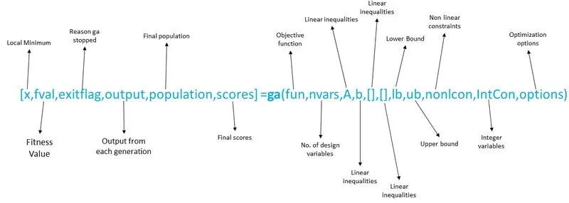
MAIN PROGRAM: To find global maxima.

clear all
close all
clc
x = linspace(0,0.6,150);
y = linspace(0,0.6,150);
num_cases = 50

[X,Y] = meshgrid(x,y);                      
for i = 1:length(X) 
    for j = 1:length(Y)
        input_vector(1) = X(i,j);
        input_vector(2) = Y(i,j);
        f(i,j) = stalagmite(input_vector);
    end
end
tic
%study case 1 statical behaviour
for i = 1:num_cases
    [inputs, fopt(i)] = ga(@stalagmite, 2);
    xopt(i) = inputs(1);
    yopt(i) = inputs(2);
end

study1_time = toc
figure(1)
subplot(2,1,1)
hold on
surfc(x,y,f)
shading interp
plot3(xopt,yopt,fopt, 'Marker','o','markersize',5,'MarkerFaceColor','r')
title('unbounded inputs')
subplot(2,1,2)
plot(fopt)
xlabel('interations')
ylabel('function minimum')

tic
%study 2 statistical behaviour - with upper and lower bounds
for i = 1:num_cases
    [inputs, fopt(i)] = ga(@stalagmite,2,[],[],[],[],[0,0],[0.5,0.5]);
    xopt(i) = inputs(1);
    yopt(i) = inputs(2);
end

study2_time = toc

figure(2)
subplot(2,1,1)
hold on
surfc(x,y,f)
shading interp
plot3(xopt,yopt,fopt, 'Marker','o','markersize',5,'MarkerFaceColor','r')
title('bounded inputs')
subplot(2,1,2)
plot(fopt)
xlabel('interations')
ylabel('function minimum')

%study 3 increasing GA iterations
options = optimoptions('ga')
options = optimoptions(options,'populationSize', 170);

tic
for i = 1:num_cases
    [inputs, fopt(i)] = ga(@stalagmite,2,[],[],[],[],[0,0],[0.5,0.5],[],[],options);
    xopt(i) = inputs(1);
    yopt(i) = inputs(2);
end

study3_time = toc

figure(3)
subplot(2,1,1)
hold on
surfc(x,y,f)
shading interp
plot3(xopt,yopt,fopt, 'Marker','o','markersize',5,'MarkerFaceColor','r')
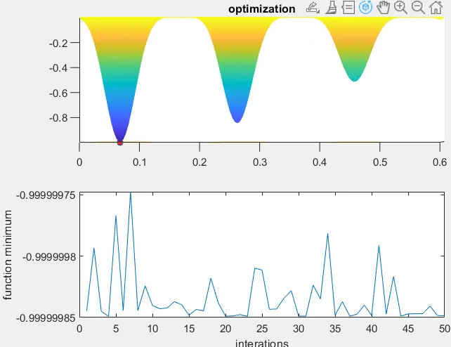
title('optimization')
subplot(2,1,2)
plot(fopt)
xlabel('interations')
ylabel('function minimum')

function [f] = stalagmite(input_vector)
x=input_vector(1);
y=input_vector(2);

f1 = (sin((5.1*pi*x)+0.5))^6;
f2 = (sin((5.1*pi*y)+0.5))^6;
f3 = exp(-4*log(2)*((x-0.0667)^2)/0.64);
f4 = exp(-4*log(2)*((y-0.0667)^2)/0.64);

f = -(f1*f2*f3*f4);
end

EXPLANATION OF PROGRAM STEP WISE:

1. Initially x and y range of 0 and 0.6 with the range of 150 and num_cases as 50.
2. We will store the x,y value in 2d arrays by using meshgrid function.
3. The function which stored is called in this code for loop function in which our output_vector is differenciated into input_vector(1) and input_vector(2).
4. The study behaviour for figure 1 with unbounded inputs includes calling our predefinrd function in a loop function and running it with our number of num_cases. The study time for 1st plot is calculated and surface plot is calculated and surface plot is employed here.The subplot defines the rows,columns and the position of the variable.
5. The study behaviour for figure 2 with bounded inputs includes calling our predefined function as in the study behaviour 1. The only difference between 1 and 2 is, the plot 2 will have different syntax of ga such that it will define along with the range of inputs.
6. The study behaviour for figure 3 with increase in options includes calling our predefined function as in both studies. The differnce among all the three studies are, in the third study we increase the population sixe so that the number of population in each generations is given as.

Thus all three figures have obtained with the given values.

num_cases = 50, It is mainly used to check the consistency of the values we are getting in the plot.

OUTPUT: Figure 1

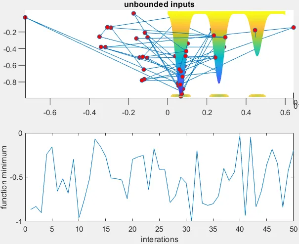
Figure 2

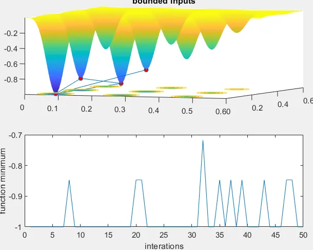
Figure 3

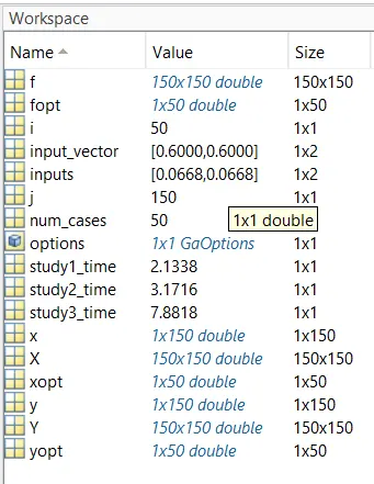
RESULTS: In workspace the result is shown

REFERENCES:

1. https://www.bing.com/ck/a?!&&p=f3e400baf8c2f9dc5078405c7861404dd497fa09909dfb8c93860b1aec261133JmltdHM9MTY1Mzk3NjUzNSZpZ3VpZD1kZjRjNTcxZC1hZWI1LTRmZmMtYmE4My1kODQzMmYxOGFjN2ImaW5zaWQ9NTIwMA&ptn=3&fclid=49b2a2c6-e0a6-11ec-9648-3a7f825f52e3&u=a1aHR0cHM6Ly93d3cudmVkYW50dS5jb20vYmlvbG9neS9zdXJ2aXZhbC1vZi10aGUtZml0dGVzdA&ntb=1
2. https://www.bing.com/ck/a?!&&p=637e2b5ec3af2e82964a53745a57973189d28fda904708af078190910a65729aJmltdHM9MTY1Mzk3NjIxNiZpZ3VpZD04NzMwYTBjNS00YTk1LTQxYWMtOTQ0OC0wMGI3NTQxNTllMGImaW5zaWQ9NTQxNQ&ptn=3&fclid=8b8b3d4c-e0a5-11ec-a224-ab6189a2c9ac&u=a1aHR0cDovL2V0aGVzaXMubml0cmtsLmFjLmluLzE5OS8xL0ZJTkFMX1JFUE9SVC5wZGYjOn46dGV4dD1UaGUlMjBHZW5ldGljJTIwQWxnb3JpdGhtJTIwaXMlMjBhJTIwcG9wdWxhciUyMG9wdGltaXphdGlvbiUyMHRlY2huaXF1ZSxiYXNpYyUyMGdlbmV0aWMlMjBvcGVyYXRvcnMlMjBvZiUyMHNlbGVjdGlvbiUyQyUyMGNyb3Nzb3ZlciUyMGFuZCUyMG11dGF0aW9uLg&ntb=1