Week 3 - Solving second order ODEs

AIM= Write a MATLAB program to solve 2nd order ODEs & that will simulate the simple pendulum motion.

OBJECTIVE:

1. To write a program to simulate the transient behaviour of a simple pendulum.
2. To create an animation of the motion of simple pendulum by using MATLAB.

THEORY

DIFFERENTIAL EQUATIONS(ODE)

A Differential Equations is an equation which contains one or more terms and derivatives of one variable(i.e.,dependent variable) with respect to the other variables (i.e.,independent variables).

First order differential equations

All the linear equation in the form of derivatives are in the first order. which has degree equal to 1. It has only the first derivatives such as `dy/dx`, where x and y are two variable.

Second order differential equations

The equation which includes the second order derivative is the second-order differential equation. It is represented as:,

`d/dx(dy/dx) = frac(d^2y)(dx^2)`

Simple Pendulum

simple pendulum is defined to have that has a small mass, also known as the pendulum bob,which is suspended from a light wire or string, as shown in the figure below.

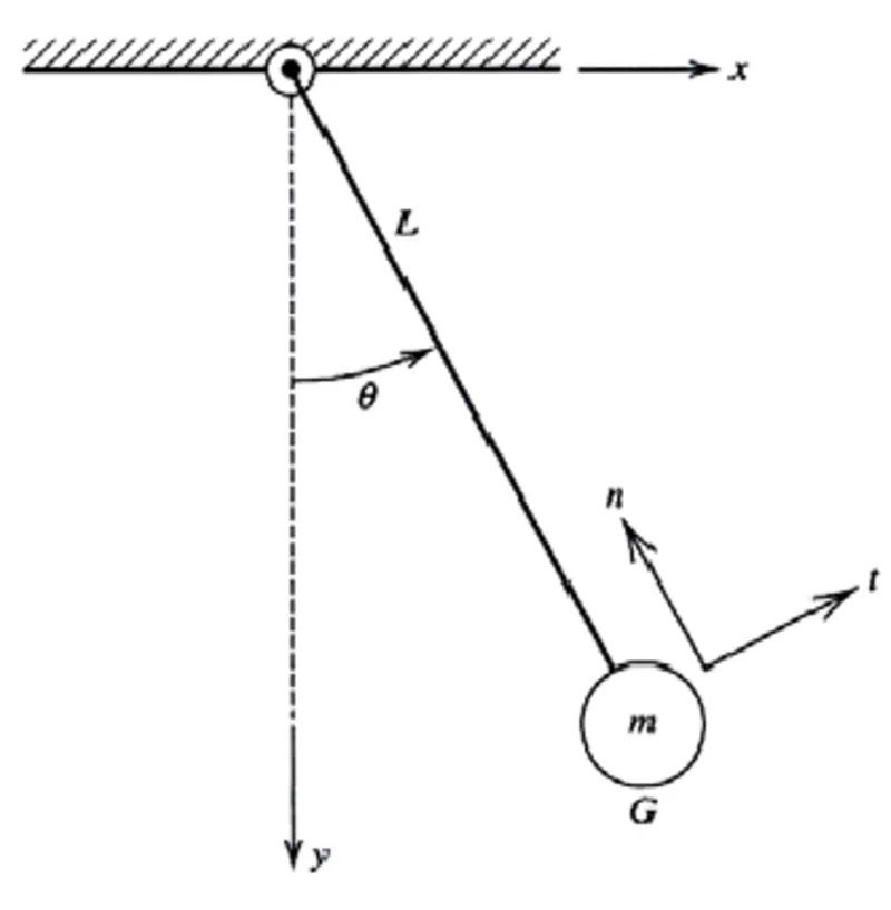
The dynamic behaviour of pendulum bob is important to understand the motion of the simple pendulum. When the pendulum bob is given an initial push while it at rest, it experiences a force sideways. It is displaced from its equilibrium position and start to oscillate . In general the motion of a simple pendulum is considered to be simple harmonic motion with constant amplitude and is given by the equation,

`frac(d^2theta)(dt^2)+g/lsintheta = 0`

where g = acceleration due to gravity in m/s^2;

`theta`= angular displacement fo the pendulum bob;

L = length in the pendulum bob in m.

Derivation for code simplification

let angular displacement `theta = theta1`, and angular velocity will be `frac(d theta)(dt) = frac(d theta1)(dt)=theta2`

`frac(d^2theta)(dt^2) = frac(d^2theta1)(dt^2) = d/dt(frac(d theta1)(dt)) = (d theta2)/dt`

Subsituting these in the second order ODE for a simple pendulum ,we get,

`frac(d^2theta)(dt^2)+b/m(d theta1)/dt+g/lsintheta1 = 0`

`frac(d^2theta)(dt^2)+b/m((d theta1)/(dt))+g/lsintheta1 = 0`

`(d theta2)/dt+b/mtheta2+g/lsintheta1`

To solve second order differential equation to break the equation in two parts . If three order then it will break 3 parts.

This is first order differential equation,hence we can write,

`therefore (d theta1)/(dt) = theta2`

`therefore (d theta2)/(dt) = -b/mtheta2-g/lsintheta1`

• Newton's second law yield linear second orderODE's

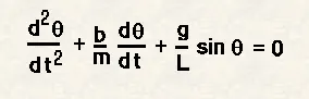
In the above equation,

Gravity (g) = 9.81 m/s^2,

Length of the pendulum (l) = 1m,

Mass of the ball (m) = 0.1kg,

Damping coefficient(b) = 0.05

Simulate the motion between 0-20 sec,

Angular displacement = 0,

Angular velocity = 3 rad/sec , at time = 0

The above inputs used in the program and get the outputs.

% Solving second order ODE pendulum equation

MATLAB PROGRAM:

clear all
close all
clc

% inputs 
b = 0.05;    
g = 9.81;
l = 1;
m = 0.1;

% initial conditions 
theta_0 = [0;5];

% time points
t_span = linspace(0,10,500);

% solve ode
[t, results] = ode45(@(t,theta)ode_function(t,theta,b,g,l,m),t_span,theta_0);

plot(t,results(:,1))
hold on 
plot(t,results(:,2))
xlabel('plot')
ylabel('time in second')

% iteration using for loop to create an animation of simple pendulum
ct = 1;
theta1 = results(:,1);

for i = 1:length(results(:,1))

  %initial conditions
  x_start = 0;
  y_start = 0;
  theta2 = theta1(i);
   
  %final conditions
  x_end = l*sin(theta2);
  y_end = -l*cos(theta2);
  
  %plotting for animation
  figure(2)
  %base of pendulum
  plot([-1 1],[0 0],'LineWidth',4,'Color','black')
  hold on
  %string of pendulum
  line([x_start x_end],[y_start y_end], 'linewidth',6,'color','b')
  %bob of pendulum
  plot(x_end,y_end,'marker','o','markersize', 28,'markerfacecolor','r')
  plot([x_start x_end],[y_start y_end],'linewidth',3)
  axis([-2 2 -2 2])
  pause(0.01)
  hold off
  M(ct)=getframe(gcf);
  ct = ct+1;
end

movie(M)
Videofile = VideoWriter('ode_function.avi','Uncompressed AVI');
open(Videofile)
writeVideo(Videofile,M)
close(Videofile)

function [dtheta_dt] = ode_function(t,theta,b,g,l,m)
theta1 = theta(1)
theta2 = theta(2)
dtheta1_dt = theta2;
dtheta2_dt = -(b/m)*theta2-(g/l)*sin(theta1);
dtheta_dt = [dtheta1_dt; dtheta2_dt];
end

EXPLANATION THE PROGRAM CODE:

1. The code start with clear all, to clear workspace, close all, to close all the plots and figures, clc to clear the command window.
2. function ode_function is created and inputs is given and run variable (l,b,g,m,t,theta).
3. The given inputs values of b,g,l,m are entered and the initial conditions for angular displacement`theta1`= 0, angular velocity`theta2`= 3rad/sec are entered to the variable'theta_0'.
4. The time span of the motion of simple pendulum 't_span' is taken to be 20sec with 500 equal intervals
5. ode45 - ode45 is an inbuilt Matlab function of choice among the ODE solvers. It compares 4th and 5th order methods to estimate error and determine step size. For differential equations with smooth solutions,ode45 is often more accurate than ode23.
6. [t,y] contains the results which we need to plot with respect to timr in which y(1) contains time in second and y(2) contains plot . Thus 'y' is an array.
7. using the results, the graph of 'time in second' and 'plot' with respect to time is plotted.
8. Then counter 'ct' is initialized. Here 'ct' is variable that simply increments by a specific step value in every step iteration of a loop.
9. To provide the continuous motion a 'for' loop the coordinates(x_start,y_start,x_end,y_end). and the increment is increase bt 1.
10. Then 'getframe' command is used to capture the motion of the lines and stored in a variable M.
11. By using 'movie' command, Matlab is going to make a movie with all the framers stored in variable M.
12. Then the video file is opened after the plot, the movie is run and after completion the video stops or closes.

OUTPUT:

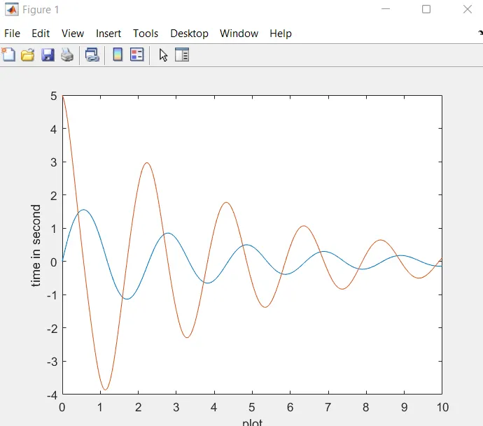
THE ANIMATION YOUTUBE VIDEO LINK:

https://youtu.be/Hr9LhQiEIIs

ERROR#1

To face some problem to create a an animation of simple pendulum.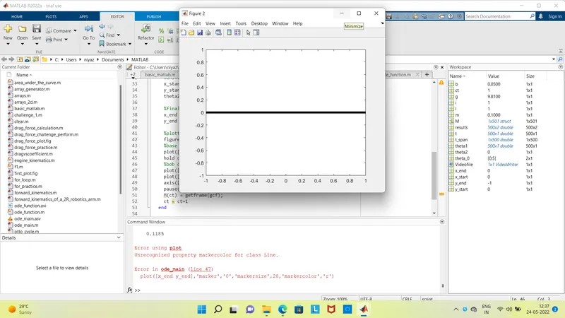

SOLUTIONS#: In line#47 put 'zero' instead of 'o' thats why the problem is facing.

RESULTS :

1. As seen in the graph, the periodic curve of angular displacement and angular velocity reduces with respect to time
2. From the animation of the motion of the simple pendulum, it can be concluded that, as the damping coefficient is increased, the motion of the pendulum reduces correspondingly and approches the equilibrium position. Also increase in damping coefficient reduces the time taken by the pendulum to reach the equilibrium position and vice-versa.