Wide Open Throttle for GM EV1 & Vehicle Propulsion Power

Wide Open Throttle Condition

AIM: To evaluate power requirements for Wide open throttle condition.

OBJECTIVES OF THE PROJECT:

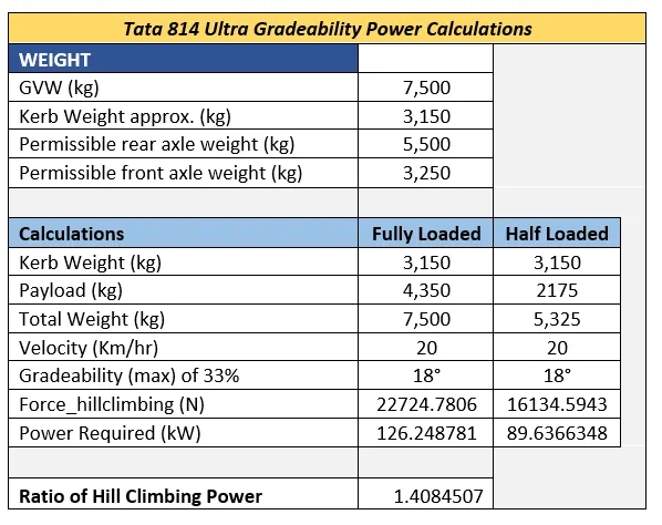
1. What is the ratio of hill-climbing power required by fully loaded tata ultra-truck to the half-loaded one?
2. A flyover is planned to be constructed on a national highway. Keeping in mind about the gradeability for trucks, how much can be the minimum length of the flyover, considering the minimum height at the summit should be 5.5 meters? State your assumptions.
3. Using Simulink glider model prepare vehicle output parameters report.
4. Model the WOT (Wide Open Throttle) response of GM EV1 car. Compare it with the official figures of the performance of a real vehicle. Prepare a table showing variation in acceleration time with a 5% change in vehicle parameters.

Objective: 1 Tata 814 Ultra

Objective 2 : Height of Flyover

Assumption:

For evaluating the length of flyover, lets assume that the heaviest truck that will climb this flyover is a BharatBenz 2823R with a working capacity of 28tons & all other vehicles that will be using this flyover have the minimum gradeability of 22%.

For evaluating minimum length of the flyover, we will assume the maximum gradeability and calculate the length of the flyover depending on the height constraints.

`Gradeability = (Height)/(Base)`

`Tanβ=(Height)/(Base`

`Tan^-1 (22%)= (Height)/ (Base`

Now, 22% Gradeability means a maximum angle of 12.4 degrees

So calculating the Length of the Flyover with minimum height of 5.5 meters and gradeability of 22%

`Sin(12.4 )=(Height)/(Flyover Leng`

`Leng of Flyover= (Height)/sin(12.4)`

`Leng of Flyover= 5.5/0.215=25.6m`

For down ward movement, lets assume the same length so total length of 50m

Objective 3: Simulink Glider Model

A driving cycle is a series of data points representing the speed of a vehicle versus time.

Driving cycles are produced by different countries and organizations to assess the performance of vehicles in various ways, as for instance fuel consumption, electric vehicle autonomy and polluting emissions.

Another use for driving cycles is in vehicle simulations. More specifically, they are used in propulsion system simulations to predict performance of internal combustion engines, transmissions, electric drive systems, batteries, fuel cell systems, and similar components.

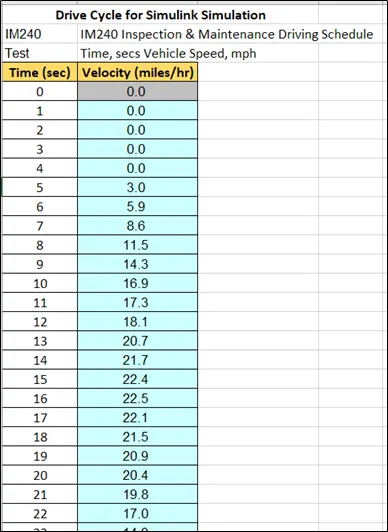
For this problem, we will be using IM240 Inspection & Maintenance Driving Schedule.

We have tabulated the values in a excel sheet, sample screenshot is attached below.

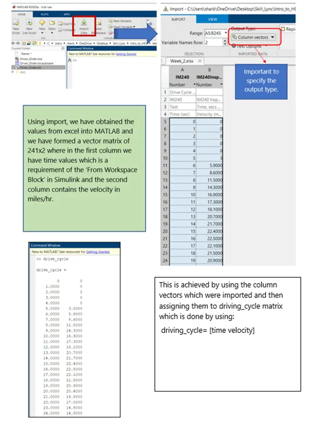
Simulink Glider Model:

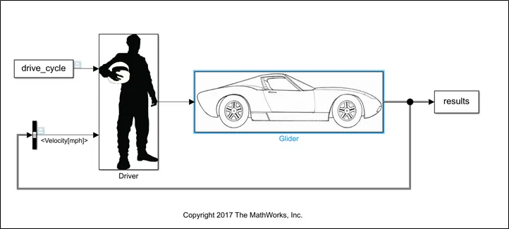
Here we are providing input using the ‘From Workspace’ block and we are using the dataset we have imported from excel.

Glider Model:

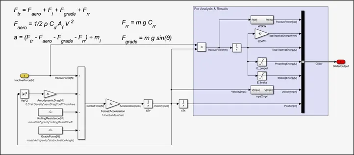
And for providing the angle of inclination we will be changing its value in the glider model as follows:

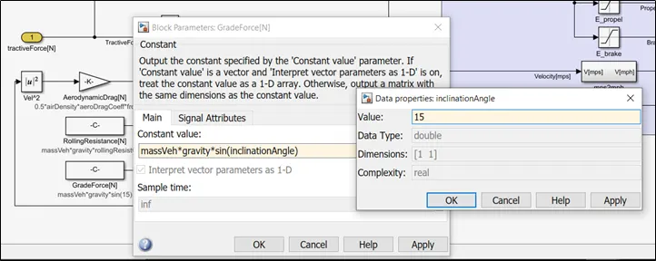
Here we are assuming a constant angle of inclination as 15 degrees.

OUTPUT:

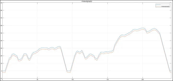
Here we can observe the velocity response with our input velocity along with time. The blue curve represents the inputs given by us and the red line refers to the response generated by the Simulink model.

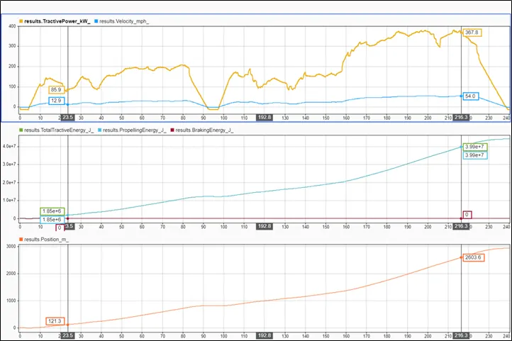
Here we can observe that the model evaluates the tractive power based on the velocity and we can also visualize the energy requirements of the vehicle along with the distance that it has travelled in the given span of time.

We can see that the model evaluates the maximum power of 367.8kW when it maneuvers to 54 miles/hr. This helps us understand the design requirements for our propulsion system.

Objective 4: WOT for GM EV1

Total tractive effort delivered by the motor:

`F_(te) = F_(rr) + F_(ad) + F_(hc) + F_(la) + F_(ωa)`

where:

• `F_(rr`is the rolling resistance force
• `F_(ad` is the aerodynamic drag
• `F_(hc` is the hill climbing force
• `F_(la` is the force required to give linear acceleration
• `F_(ωa`is the force required to give angular acceleration to the rotating motor

Acceleration figures are found from simulation or testing of real vehicles. For IC engine vehicles this is done at maximum power, or ‘wide open throttle’ (WOT). Similarly, for electric vehicles performance simulations are carried out at maximum torque.

that the maximum torque of an electric motor is a fairly simple function of angular speed.

In most cases, at low speeds, the maximum torque is a constant, until the motor speed reaches a critical value ωc after which the torque falls.

For `ω<r*Gω_c`, orthen `T = T_max`

Once this constant torque phase is passed, i.e. `ω ≥ ω_c`, or `v >= r* ω_c/G` then either the power is constant, or the torque falls.

For a vehicle on level ground, with air density 1.25 kg.m−3

`(G/r)* T = µ_(rr)*m*g + 0.625*A*C_d* ν^2 + ( m + (I *G^2)/ ηg*r^2) (dν)/dt`

Modelling of GM EV1

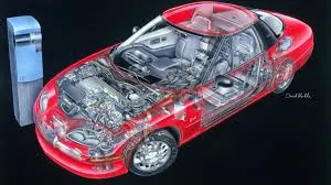
The GM EV1 was arguably the first modern electric car from one of the really large motor companies.

`C_d =0.19`

`µ_(rr) = 0.0048`

Total Mass of Vehicle considering the passengers and component mass =1540 Kg

The motor’s moment of inertia is not known, however, compared to the mass of such a heavy vehicle this will be very low; the wheels are also very light and we will approximate this term by increasing the mass very modestly to 1560 kg in the final term of equation.

`G=11`

Radius of tire=0.3 m

The use of variable frequency induction motors, operating at very high speed, nearly 12 000 rpm at maximum speed.

`T_max=140 Nm`

`ω_c = 733 rad*s^(−1` note this means `T = T_max` until v = 19.8 ms−1 (= 71.3 kph);

above 19.8 ms−1 the motor operates at a constant 102 kW, as this is a WOT test, so:

`T = 102000 /(37 × v) = 2756/ v`

Frontal Area `A = 1.8 m^2`

`η_g = 0.95`

Hence substituting these values in our equation:

`(G/r)* T = µ_(rr)*m*g + 0.625*A*C_d* ν^2 + ( m + (I *G^2)/ η_g*r^2) *(dν) /dt`

`0.95 × 37 × 140 = 72.4 + 0.214v^2 + 1560 (dν )/dt`

`So,(dν)/dt = 3.11 − 0.000137*v^2`

Once the speed has reached 19.8 ms−1 the velocity is given by the differential equation:

`(0.95 × 37 × 2756 )/ν = 72.4 + 0.214*v^2 + 1560 (dv)/dt`

`So,(dv)/dt = 62.1/v − 0.046 − 0.000137*v^2`

`v_(n+1) = (v_n + ∂t)*(3.11 − 0.000137*v_n^2)`

`v_(n+1) = (v_n + ∂t) *(62.1/v_n − 0.046 − 0.000137*v_n^2)`

MATLAB CODE for Generating the WOT Velocity variation :

%Modelling WOT for GM EV1 
close all
clear all
clc
time=linspace(0,30,301); %Array containing time values
vel=zeros(1,301); %initializing storage for velocity values
distace=zeros(1,301); %initializing storage for distance values
dT=0.1;
for n=1:300
if vel(n)<19.8      %19.8m/sec is the critical velocity for the motor
   vel(n+1) = vel(n) + dT*(3.11 + (0.000137*(vel(n)^2)));
elseif vel(n) > 35.8
% Controller stops any more speed increase
vel(n+1) = vel(n);
else
vel(n+1) = vel(n) + dT * ((62.1/vel(n)) - 0.046 - (0.000137*(vel(n)^2)));
%Calculating the distance 
distace(n+1)=distace(n)+0.1*vel(n); 
end
end
%Plotting initial results 
vel=vel*3.6; %converting velocity to km/hr
figure(1)
plot(time,vel,'linewidth',3,'color','green');
xlabel('Time(sec)')
ylabel('Velocity Km/hr')
title('WOT for GM EV1')
grid on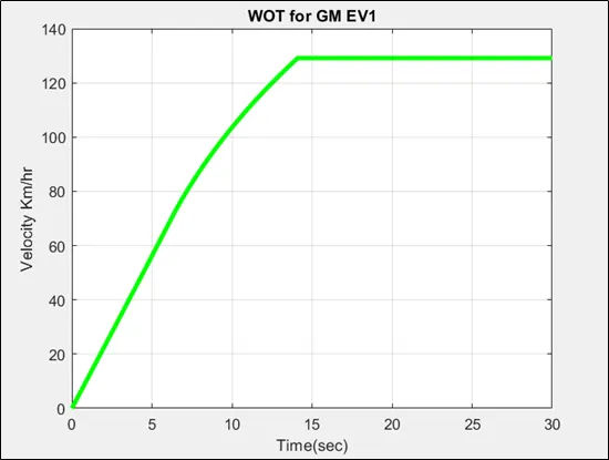

Official figures for GM Ev1:

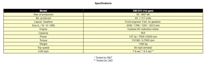
So, we can observe that our data matches the results obtained by us. we can see that the time taken to reach 96 kph, which is 60mph, is just under 9 s. Not only is this a very respectable performance, but it is also exactly the same as given in the official figures for the performance of the real vehicle.

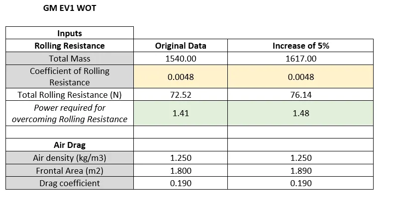
For variation of 5% in parameters:

%For variating with 5% increase 
velnew=zeros(1,301); %%initializing storage for velocity values
for n=1:300
if velnew(n)<19.8      %19.8m/sec is the critical velocity for the motor
   velnew(n+1) = velnew(n) + dT*(2.85 + (0.00013*(velnew(n)^2)));
elseif velnew(n) > 35.8
% Controller stops any more speed increase
velnew(n+1) = velnew(n);
else
velnew(n+1) = velnew(n) + dT * ((57.05/velnew(n)) - 0.044 - (0.000132*(velnew(n)^2)));
%Calculating the distance 
distace(n+1)=distace(n)+0.1*velnew(n); 
end
end

%Plotting Comparision 
velnew=velnew*3.6; %converting velocity to km/hr
figure(2)
plot(time,vel,'linewidth',1,'color','green');
hold on 
plot(time,velnew,'linewidth',2,'color','blue');
xlabel('Time(sec)')
ylabel('Velocity Km/hr')
legend('Original','With 5% icrement')
title('WOT for GM EV1 comparison')
grid on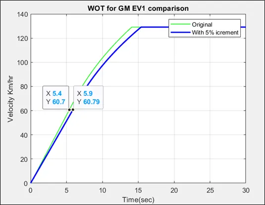

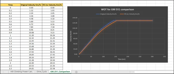
A same comparison is done in excel and attached for reference.

CONCLUSION:

1. A power ratio of 1.4 was obtained between fully loaded and half loaded Tata Ultra 814 series truck.
2. For the data given for flyover, we found that for the height of 5.5 meters we need a flyover having a length of 50 metres.
3. Using IM240 Inspection & Maintenance Driving Schedule for the Simulink model we established the propulsion power required by the electric motor.
4. Wide open throttle characteristics for GMEV1 were observed.

RESOURCES:

MathWorks Student Competitions Team (2020). MATLAB and Simulink Racing Lounge: Vehicle Modeling (https://www.mathworks.com/matlabcentral/fileexchange/63823-matlab-and-simulink-racing-lounge-vehicle-modeling), MATLAB Central File Exchange. Retrieved September 18, 2020.

Excel Link for Reference