Optimization of Stalagmite Function using Genetic Algorithm

AIM: To write a code in MATLAB to optimize the stalagmite function and find the global maxima of Stalgamite Function

OBJECTIVES OF THE PROJECT:

1. Explore the concept of Genetic Algorithm in MATLAB
2. Optimize Stalagmite function & study its Statistical Behavior based on search space & population size of the initial search space

WORKFLOW:

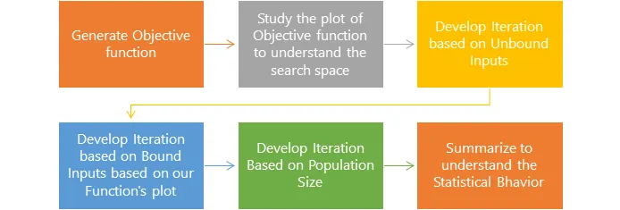
Genetic Algorithm

A genetic algorithm (GA) is a method for solving both constrained and unconstrained optimization problems based on a natural selection process that mimics biological evolution.

You can apply the genetic algorithm to solve problems that are not well suited for standard optimization algorithms, including problems in which the objective function is discontinuous, nondifferentiable, stochastic, or highly nonlinear.

In computer science and operations research, a genetic algorithm (GA) is a metaheuristic inspired by the process of natural selection that belongs to the larger class of evolutionary algorithms (EA). Genetic algorithms are commonly used to generate high-quality solutions to optimization and search problems by relying on biologically inspired operators such as mutation, crossover and selection

The process of natural selection starts with the selection of fittest individuals from a population. They produce offspring which inherit the characteristics of the parents and will be added to the next generation. If parents have better fitness, their offspring will be better than parents and have a better chance at surviving. This process keeps on iterating and at the end, a generation with the fittest individuals will be found.

This notion can be applied for a search problem. We consider a set of solutions for a problem and select the set of best ones out of them.

Five phases are considered in a genetic algorithm.

1. Initial population
2. Fitness function
3. Selection
4. Crossover
5. Mutation

How the Algorithm Works

The following outline summarizes how the genetic algorithm works:

1. The algorithm begins by creating a random initial population.
2. The algorithm then creates a sequence of new populations. At each step, the algorithm uses the individuals in the current generation to create the next population. To create the new population, the algorithm performs the following steps:
   1. Scores each member of the current population by computing its fitness value. These values are called the raw fitness scores.
   2. Scales the raw fitness scores to convert them into a more usable range of values. These scaled values are called expectation values.
   3. Selects members, called parents, based on their expectation.
   4. Some of the individuals in the current population that have lower fitness are chosen as elite. These elite individuals are passed to the next population.
   5. Produces children from the parents. Children are produced either by making random changes to a single parent—mutation—or by combining the vector entries of a pair of parents—crossover.
   6. Replaces the current population with the children to form the next generation.
3. The algorithm stops when one of the stopping criteria is met.

Syntax of Genetic Algorithm for MATLAB

[x,fval] = ga(fun,nvars,A,b,[],[],lb,ub,nonlcon,IntCon,options)

1. ‘ga’ stands for ‘Genetic algorithm’
2. ‘x’ is the array containing the value of co-ordinates at which the minimum value of the function being optimized is evaluated by ‘ga’.
3. ‘fval’ is the minimum value of the function obtained by ga
4. ‘fun’ is the function being optimized
5. ‘nvars’: is the number of iterations the algorithm shall work
6. ‘A,b’ :Used when the function is subjected to the linear inequalities A*x ≤ b. ga evaluates the matrix product A*x as if x is transposed (A*x')
7. ‘Aeq,beq’ : Used when the function is subjected to the linear equalities Aeq*x = beq and A*x ≤ b. (Set A=[] and b=[] if no linear inequalities exist.) ga evaluates the matrix product Aeq*x as if x is transposed (Aeq*x').
8. ‘Lb,ub’ : defines a set of lower and upper bounds on the design variables, x, so that a solution is found in the range lb ≤ x ≤ ub. (Set Aeq=[] and beq=[] if no linear equalities exist.)
9. ‘nonlcon’: subjects the minimization to the constraints defined in nonlcon. The function nonlconaccepts x and returns vectors C and Ceq, representing the nonlinear inequalities and equalities respectively. ga minimizes the fun such that C(x) ≤ 0 and Ceq(x) = 0. (Set lb=[] and ub=[] if no bounds exist.)
10. ‘options’ : minimizes with the default optimization parameters replaced by values in options. (Set nonlcon=[] if no nonlinear constraints exist.) Create options using optimoptions.

We will be using MATLAB CODE to optimize Stalagmite Function:

Stalagmite function:

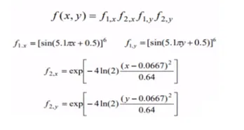
%%Defining Objective Function 
function z=stalagmite(input_vector)
x=input_vector(1); % defining inouts x
y=input_vector(2); % defining inouts y

%Term 1
f1x=(sin((5.1*pi*x)+0.5))^6;
%Term 2
f2x=exp(-4*log(2)*((x-0.0667)^2)/0.64);

%Term 3
f1y=(sin((5.1*pi*y)+0.5))^6;
%Term 4
f2y=exp(-4*log(2)*((y-0.0667)^2)/0.64);

%Stalagmite function is function of all the terms 
z=-(f1x*f2x*f1y*f2y);   
end

Explanation:

1. Code for the stalagmite function contains 4 terms, each term is coded separately according to function definition.
2. The input for the stalagmite function is taken as row vector which contains two columns representing the values of x and y.
3. Finally, as the stalagmite function is a function of all these terms, we represent ‘z’ as the stalagmite function which is a product of all these terms.
4. A negative sign is used as ‘ga’ evaluates minimum of the function and we are interested in finding the maximum value for the function.

Code for Statistical behavior:

%Using Genetic Algorithm to obtain Maximum value of Stalagmite Function

close all
clear all
clc
%%
%%Defining Inputs for Stalagmite Function
x=linspace(0,0.6,150);
y=linspace(0,0.6,150);
[xx,yy]=meshgrid(x,y);  %Creating a 2-Dimensional grid from 1D Array

%%
%Evaluating Stalagmite function
for i=1:length(xx);
    for j=1:length(yy);
        input_vector(1)=xx(i,j);     %Defining input-vector for Stalagmite Function
        input_vector(2)=yy(i,j);     %Defining input-vector for Stalagmite Function

    z(i,j)=stalagmite(input_vector);         %Evaluating Stalagmite Function
    end
end
%%
%Defining number of Iterations for Genetic algorithm
n=50;

tic    %Starting Time Counter
%Study 1: Statistical Behavior of Stalagmite Function "Unbound"
for i=1:n;
[co_out,fval(i)]=ga(@stalagmite,2); %using 'ga' to evaluate minimum based on Genetic algorithm
x_out(i)=co_out(1);      %value of x coordinate for predicted value by ga
y_out(i)=co_out(2);      %value of y coordinate for predicted value by ga
end
t1=toc  %Ending Time Counter
%Plotting
figure(1)
subplot(2,1,1)
surfc(xx,yy,-z);    %Plotting Stalgamite function
xlabel('X-Axis');
ylabel('Y-Axis');
shading interp      %Interpolated representation 
hold on 

%Plotting ga results 
plot3(x_out,y_out,-fval,'-o','markersize',5,'markerfacecolor','r');
title('Statistical Behavior of Stalagmite Function "Unbound"')
subplot(2,1,2)
plot(-fval);
xlabel('Iterations')
ylabel('Optimum Value of Function')
%%
tic        %Starting Time Counter
%Study 2 :  Statistical Behavior on Providing Lower bound & Upper Bound 
%Changing Search range for ga 
lb=[0;0];   %lower bound on function value predicted by ga
ub=[1;1];   %Upper bound on function value predicted by ga
for i =1:n ;
   %Syntax : x = ga(fun,nvars,A,b,Aeq,beq,lb,ub)
   [co_out_1,fval_1(i)]=ga(@stalagmite,2,[],[],[],[],lb,ub);
   x1_out(i)=co_out_1(1); %value of x coordinate for predicted value by ga
   y1_out(i)=co_out_1(2); %value of y coordinate for predicted value by ga
end

t2=toc  %Ending Time Counter

%Plotting
figure(2)
subplot(2,1,1)
surfc(xx,yy,-z);    %Plotting Stalgamite function
xlabel('X-Axis');
ylabel('Y-Axis');
shading interp      %Interpolated representation 
hold on 

%Plotting ga results 
plot3(x1_out,y1_out,-fval_1,'-o','markersize',5,'markerfacecolor','r');
title('Statistical Behavior: Lower bound & Upper Bound ')
subplot(2,1,2)
plot(-fval_1);
xlabel('Iterations')
ylabel('Optimum Value of Function')

%%
tic       %Starting Time Counter
%Study 3: Statistical behavior for Ga with increased population size

options=optimoptions(@ga,'populationsize',300);
for i=1:n;
   [co_out_2,fval_2(i)]=ga(@stalagmite,2,[],[],[],[],lb,ub,[],options);
   x2_out(i)=co_out_2(1);
   y2_out(i)=co_out_2(2);
end

t3=toc  %Ending Time Counter

%Plotting
figure(3)
subplot(2,1,1)
surfc(xx,yy,-z);%Plotting Stalgamite function
xlabel('X-Axis');
ylabel('Y-Axis');
shading interp      %Interpolated representation 
hold on 

%Plotting ga results 
plot3(x2_out,y2_out,-fval_2,'-o','markersize',5,'markerfacecolor','r');
title('Statistical behavior with Increased population size')
subplot(2,1,2)
plot(-fval_2);
xlabel('Iterations')
ylabel('Optimum Value of Function')


%Summary 
X_Coordinates=[x_out(50);x1_out(50);x2_out(50)];    %Column_1 of the Table
Y_Coordinates=[y_out(50);y1_out(50);y2_out(50)];    %Column_2 of the Table
Maximum_Value_predicted=[-fval(50);-fval_1(50);-fval_2(50)];    %Column_3 of the Table
time_taken_by_ga=[t1;t2;t3];     %Column_4 of the Table
row_names={'Unbound';'Upper & Lower Bound on Fval';'Increased Iterations'}; %Defining Row Names
%Defining Table 
t=table(X_Coordinates,Y_Coordinates,Maximum_Value_predicted,time_taken_by_ga,'RowNames',row_names)

Explanation:

1. Inputs for the Stalagmite function is defined using a 2D array. We used meshgrid for this purpose.
2. Using the values of xx and yy from the 2-D array, we obtain the input vectors for the stalagmite function.
3. Using a For loop we evaluate the Stalagmite function at all the values of xx and yy.
4. Number of iterations for the ga is defined as 50
5. For Study 1: we have no bounds on the search space, we simply evaluate the optimum value of the function by using the genetic algorithm
   1. In study 1 we are trying to understand the way the algorithm is predicting the values and visualize it using plot3 command.
   2. We can also check the time required for the ‘ga’ to finish the iterations
6. For Study 2: We use upper and lower bounds to define the search space for the algorithm.
   1. This is done to narrow down the search space and improve the quality of solution, this can be only done when we understand the physics of the problem we are trying to optimize, i.e we should be able to predict the solution range by understanding the nature of the solution.
   2. We plot the optimum value predicted by the solver using plot3 command along with the surface plot of the stalagmite function.
   3. To observe the convergence, we also plot the value of function for each iteration.
7. For Study 3: We use upper and lower bounds as well as we increase the population size to 300 as we want he Ga to generate more number of guesses at the initiation step so that its able to generate more mutations and hence is able to predict the optimum value at the end of the iterations for each iteration no matter how many times we run the algorithm.
   1. Here along with the bounds on the search space we are also increasing the population size at the initiation of ‘ga’
   2. x = ga(fun,nvars,A,b,Aeq,beq,lb,ub,nonlcon,options) minimizes with the default optimization parameters replaced by values in options. (Set nonlcon=[] if no nonlinear constraints exist.) Create options using optimoptions.
   3. Using : options=optimoptions(@ga,'populationsize',300) we increase the population size which is 50 by default to 300.
   4. We also plot the values predicted for each iteration.
8. Using tic and toc command we are also evaluating the time required to run the ‘ga’ for all the studies.
9. At the end we use table to summarize the results obtained.

OBSERVATION:

Study 1:

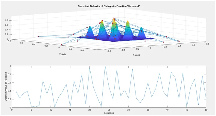
1. We can observe that the predicted optimum values are all over the place. The reason for this scattering is because we haven’t defined any particular search space for genetic algorithm hence it throws random minimum values which are not in the search space.
2. The time taken by the ‘ga’ is 2.8 seconds.

Study 2:

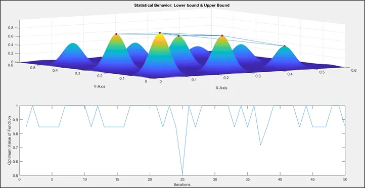
1. Here we can see that the values predicted by the genetic algorithm is better than previous case.
2. Here the values predicted are lying between Zero and One which are the lower and upper bounds respectively.
3. But this gives different results every time we run the algorithm.
4. The time taken by the ‘ga’ is 3.82 seconds.

Study 3:

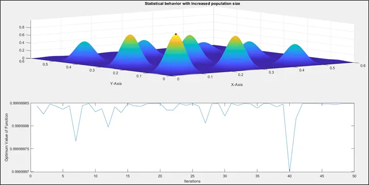
1. We can see that the values predicted by the genetic algorithm converges well.
2. It fluctuates once but than all other iterations are predicting the same value.
3. The time taken by the ‘ga’ is 16.81 seconds.

SUMMARY:

CONCLUSION:

The maximum value of the function predicted by Genetic Algorithm for Stalgamite Function is 1 at x=0.066 and y=0.066