Week 9 - Senstivity Analysis Assignment

Aim:- Write a code that calculates 10 most sensitivity values of temperature, for a given GRI30 mechanism file. The sensitivity parameter should be with respect to the temperature.

Sensitivity Analysis:- Sensitivity analysis is the study of how the uncertainty in the output of a mathematical model or system can be divided and allocated to different sources of uncertainty in its inputs. It is used to identify the parameters that affect a compound solution.

In a reaction mechanism, the change of the value of parameters in different for different reactions, which means the parameters are sensitive to some reactions and insensitive to some other reactions.

The sensitivity analysis is done by finding the slope at each time step, for each reaction. In this challenge the sensitivity analysis is done for temperature. Here the sensitivity value can be negative too, which means that the independent variable increases and dependent variable decreases.

Given:

Initial conditions are temperature - 1500K, pressure - 1atm.

Code:-

import matplotlib.pyplot as plt 
import sys 
import numpy as np
import cantera as ct

gas = ct.Solution('gri30.xml')
temp = 1500
pres = ct.one_atm

gas.TPX = temp,pres, 'CH4:1, O2:2, N2:7.52'
r = ct.IdealGasConstPressureReactor(gas)
sim = ct.ReactorNet([r])
n = gas.n_reactions
N = 10

# enable sensitivity wrt the rates of the first 10
# reactions (reactions 0 through 9)

for i in range(n):
	r.add_sensitivity_reaction(i)

# Set the tolerances for the solution and for the sensitivity coefficients
sim.rtol = 1.0e-6  # relative change in solution should be less than this number
sim.atol = 1.0e-15 # absolute change in solution should be less than this number

sim.rtol_sensitivity = 1.0e-6	# relative change
sim.atol_sensitivity = 1.0e-6	# absolute change

sT_m = [0]*n
states = ct.SolutionArray(gas, extra=['time_in_ms','t'])

for t in np.arange(0, 2e-3, 5e-6):
	sim.advance(t)
	states.append(r.thermo.state, time_in_ms=1000*t, t=t)

	for j in range(n):
		sT = sim.sensitivity('temperature', j)	
		if np.abs(sT)>= np.abs(sT_m[j]):
			sT_m[j] = sT

s_plot = []
s = np.zeros((N))

print('10 Most sensitivity reactions')
print('%8s %4s %4s %3s %4s' %('Reaction ID','|','sensitivity', '|', 'Reaction'))

for m in range(N):
	maximum = np.max(sT_m)
	minimum = np.min(sT_m)
	if np.abs(maximum)>np.abs(minimum):
		s[m] = maximum
		Reaction_index = sT_m.index(maximum)
		s_plot.append(sim.sensitivity_parameter_name(Reaction_index))
		print('%7d %8s %10.4f %4s %26s'%(Reaction_index,'|',maximum,'|',s_plot[m]))
		sT_m.remove(maximum)

	else:
		s[m] = minimum
		Reaction_index = sT_m.index(minimum)
		s_plot.append(sim.sensitivity_parameter_name(Reaction_index))
		print('%7d %8s %10.4f %4s %26s'%(Reaction_index,'|',minimum,'|',s_plot[m]))
		sT_m.remove(minimum)

for k in range(N):
	s_plot[k] = s_plot[k].replace('IdealGasConstPressureReactor_1:','')

reactions = list(reversed(s_plot))
sensitivity = list(reversed(s))

# plotting
plt.figure(1)
plt.subplot(2,2,1)
plt.plot(states.t, states.T,linewidth=2)
plt.xlabel('Time',fontweight='bold')
plt.ylabel('Temperature',fontweight='bold')
plt.grid('both',linestyle='--')
plt.subplot(2,2,2)
plt.plot(states.t, states('OH').X,linewidth=2)
plt.xlabel('Time',fontweight='bold')
plt.ylabel('OH Mole fraction',fontweight='bold')
plt.grid('both',linestyle='--')
plt.subplot(2,2,3)
plt.plot(states.t, states('O2').X,linewidth=2)
plt.xlabel('Time',fontweight='bold')
plt.ylabel('O2 Mole fraction',fontweight='bold')
plt.grid('both',linestyle='--')
plt.subplot(2,2,4)
plt.plot(states.t, states('CH4').X,linewidth=2)
plt.xlabel('Time',fontweight='bold')
plt.ylabel('CH4 Mole fraction',fontweight='bold')
plt.grid('both',linestyle='--')
plt.tight_layout()

plt.figure(2)
plt.barh(reactions,sensitivity,color='red',height=0.5)
plt.xlabel('Sensitiity values')
plt.ylabel('10 Top sensitivity reactions')
plt.title('10 Most sensitivity reactions with Temperature')
plt.show()

Result:-

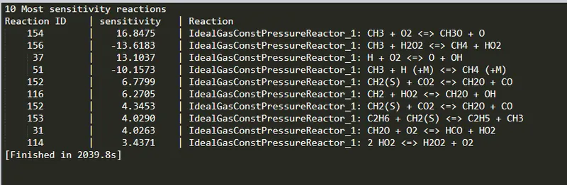
Plots:-

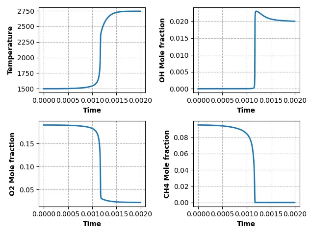
From the above images, the 1st plot shows the variation of temperature with respect to time which can be used to calculate the ignition-delay time. And the remaining 3 plots show the change in concentration of species OH, `O_2`, and `CH_4`.

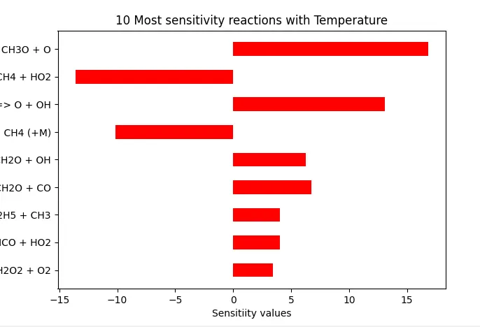
In the sensitivity analysis with respect to temperature. From the above bar, the reaction `CH_3 + O_2 iff CH_3O + O` has the most positive sensitive value, which means that the increase in the rate of this reaction or any positive value would be seeing by decreases in the ignition delay.

On the other hand, the reaction `CH_3 + H_2O_2 iff CH_4 + H_2O` has the most negative sensitive value, which means the ignition-delay is high due to low temperature.