Week - 9 Material modeling from raw data
Objective : To create a material property card using the given data, and verifying the material properties by assigning it to the dogbone specimen and studying its simulation behaviour.
Procedure :
Extraction of data :
Using the getdata application, the co-ordinates of the curve are plotted and pasted in an excel sheet.
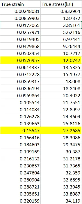
The values of strain are converted from percentage to absolute value and the value of stress is converted from ksi to Gpa.
Next we plot the graph using the true stress and strain values in Gpa and absolute values respectively.
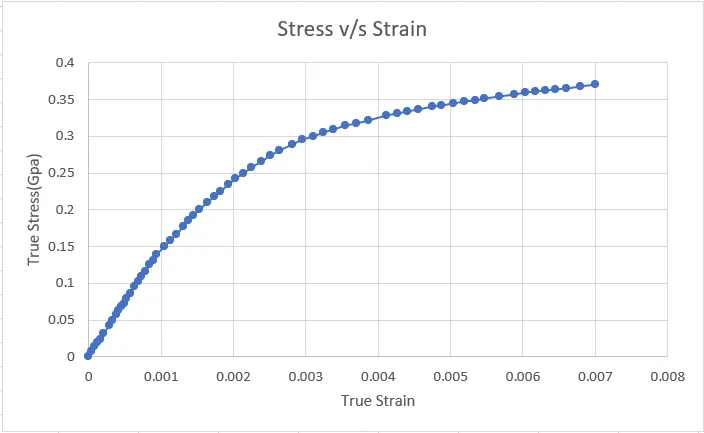
We next calculate the Young's modulus by calculating the slope of the elastic region of the curve, using the slope function in excel. We select the points in the elastic region of the curve for the calculation of E. The youngs modulus is calcluated at 147.3973 Gpa.
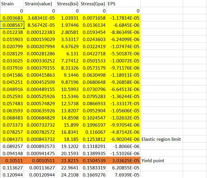
Next we calculate the values of Effective plastic strain using the formula EPS = True plastic strain - (True stress/E)
The yield point is taken as the value of stress where the EPS value switches from negative to positive. As we can see the yield point is obtained at 0.1504539 Gpa.
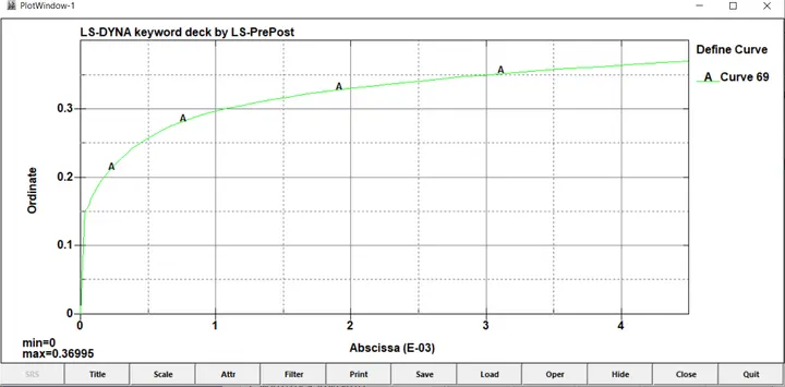
Now we will create the data table for Effective Plastic Strain (EPS) vs effective Stress (ES). The values are taken from the yield point onwards and saved in .csv format
Creation of material Card
Now we will create the material card. Go to keyword manager-->MAT-->Type 24 as shown below.
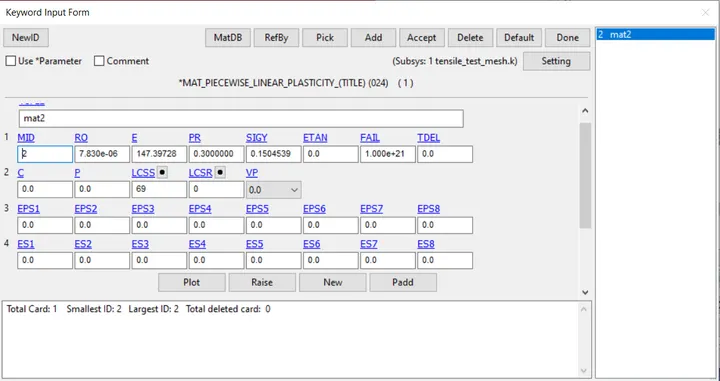
The Load curve ID is created by loading the data in the .csv file created earlier (loadcurve1) and is assigned to the material card created above. Values of yield stress, young's modulus are entered as were calculated from the data. Generic values of density and Poisson's ratio are taken and input according to the unit system (kg, mm, ms).
Setting up rest of the simulation
Boundary conditions :
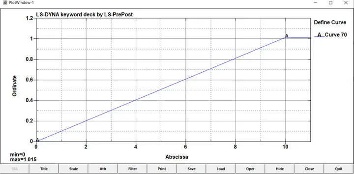
Prescribed motion is applied at one end of the dogbone specimen of the order of 1.105mm which makes the strain 0.7% as is given in the curve. The following displacement curve is used.
SPCs :
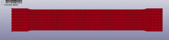
The nodes at the other end are restricted along x & z axes.
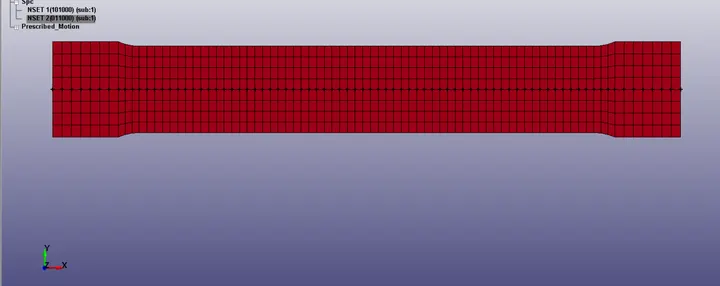
The nodes along the center line are restricted along y & z axes to constrain the neutral axis.
Creation of part :
The section ID and material ID are assigned to the part.
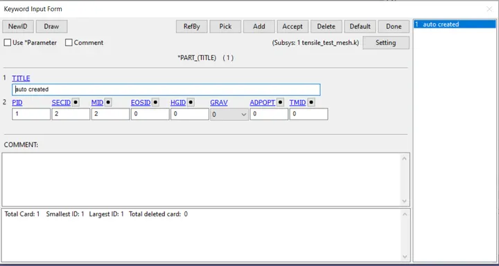
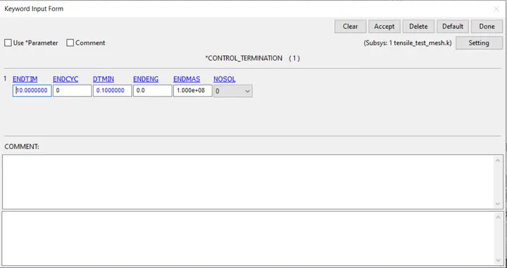
Control parameters :
The termination time is set at 10 ms.
Database options :
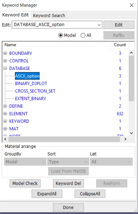
The following options are selected in the database for output of data.
Running the simulation :
Stress plots :
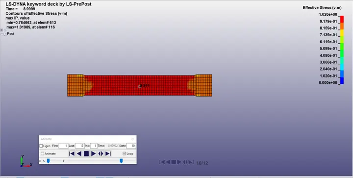
Maximum stress is obtained at 1.02 Gpa
Since we have given prescribed motion for the loading condition, we will not look at the strain contours in the simulation.
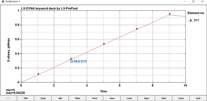
Next we pick an element in the middle of the dogbone and ontain the stress and strain plots of it, We will study the stress and strain plots at 3 ms as the specimen experiences a stress at that point in time which lies in the range of our inputted load curve for the material. The stress obtained at 3ms is around 0.317 Gpa as seen below.
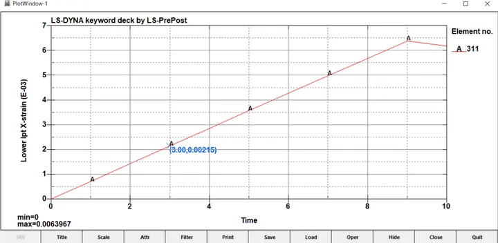
Now we study the strain curve at the same point in time of 3ms. We see that the strain at 3 ms is 0.00215.
Next we will directly correlate these 2 values with our inputted curve and see if it matches so that our result can be verified.
Verification with input data :
Looking at the input Effective stress v/s Effective Plastic Strain Curve we see that at a strain of 0.00215, the stress value of the test data is around 0.334 Gpa. The result of stress obtained during the simulation at this strain value is 0.317 Gpa. So the deviation in result is 0.317/0.334 = 0.95, which gives us 95% percent accuracy.
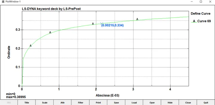
The accuracy of result may further be improved by reducing the timestep thereby refining the curve and giving us a more accurate result.
Conclusion : Hence the material card was created according to the curve provided and the result was verified in the simulation as well.
Result : Contains .k file, excel for calculations, .csv file for inputed load curve in material card.