Week - 9 Material Modeling from Raw Data
Aim :
Use the diagram of the true stress-strain curve of graphite iron casting. Two curves are there for different material structures. Students need to pick any one of them and use the data to create either a MAT_024 or MAT_018 material model and then validate it.
Solution :
It is very important to convert the material data into a material law that the solver can understand.To model the linear behaviour of a material we just need the density , youngs modulus and poisson ratio.LS Dyna consists of the following materials cards as shown below :
1.Elastic
a.Linear : Isotropic (MAT00)
b.Non Linear : Hyperelastic(MAT*077):Orthod aniso trophic :Their properties changes with direction.
2.Elastic -Plastic :These can rate dependent or rate independent .The following laws are used :
a.MAT003:PLASTIC KINEMATIC:
b.MAT0012:Isotropic Elastic Plastic:
c.MAT0015:Mat_Johnson_Cook:This considers the thermal and damage effects.
d.MAT098:Simplified_Johnson_Cook: This does not consider the thermal and damaging effects.
The following material cards are used the most to model metals :
mat_024,mat_18 and mat098
3.For a rigid material we can use mat 20
Elastic materials can be defined as shown below :
Strain rate is the rate of deformation caused by strain in a material within a corresponding time. This gauges the rate where distances of materials change within a respective period of time.
In order to input the model the material we have to convert the engineering stress -strain into true stress and strain by the following formula :
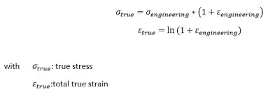
Once we get the true stress strain curve we convert it into plastic strain curve and feed this data into the material modelling.
Now we will discuss about hyperelastic material :
Hyperelastic material models are regularly used to represent the large deformation behavior of materials with FEA. They are commonly used to model mechanical behaviors of unfilled/filled elastomers. In addition to elastomers, hyperelastic material models are also used to approximate the material behavior of biological tissues, polymeric foams, etc.
Linearly elastic materials are described through two material constants (like Young’s modulus and Poisson ratio). In contrast, hyperelastic materials are described through a strain-energy density function. The strain-energy density can be used to derive a nonlinear constitutive model (i.e., stresses as a function of large strain deformation measures like deformation gradient or Cauchy-Green tensors, etc.). There are several models proposed in the literature such as the Neo-Hookean, Mooney-Rivlin and Signorini models,
Step 1: Extraction of data
The data digitizer tool is used to extract the data from curve 2 of the image given.
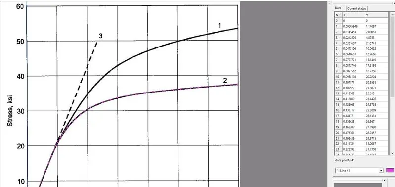
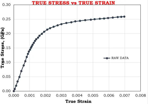
These data points, which represent the true stress - strain values are exported to an excel sheet, and the values of true stress and strain are plotted.
Step 2: Model setup in LS Dyna
1. Model import and boundary conditions
The given dogbone specimen model is imported into LS Dyna.
SPC
The boundary conditions are given as shown below.
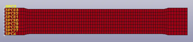
The nodes on the left edge of the specimen and constrained in the X and Z directions. They are not constrained in the Y - direction, since the speciment undergoes lateral elongation during the test.

The middle nodes on either edge are constrained in the Y - directions.
Prescribed motion
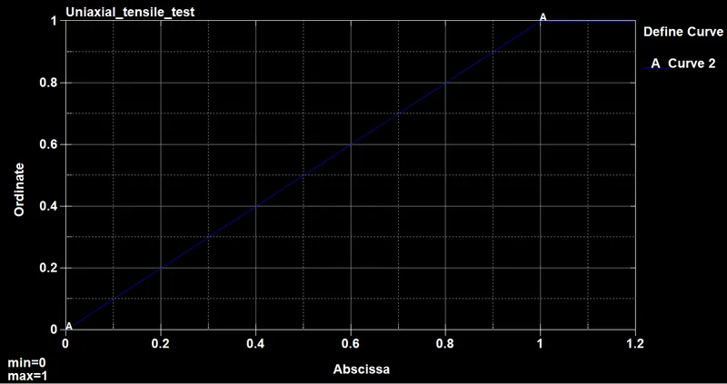
A displacement is given to the nodes at the right edge of the specimen as shown below.

2. Model definition
Section definition
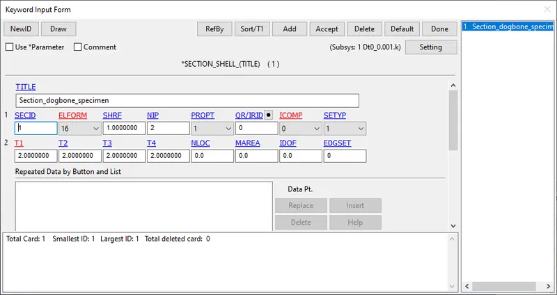
The dogbone specimen is defined with shell elements of thickness 2mm and ELFORM 16 as shown below.
Material Definition
The MAT 24 piecewise linear card is defined with the following parameters. The unit system used is kg-mm-ms. The Young's modulus (E) is 20.9 e+6 psi which is 144.100 Gpa. The value of density (RO) and poisson's ratio (PR) are given accordingly.
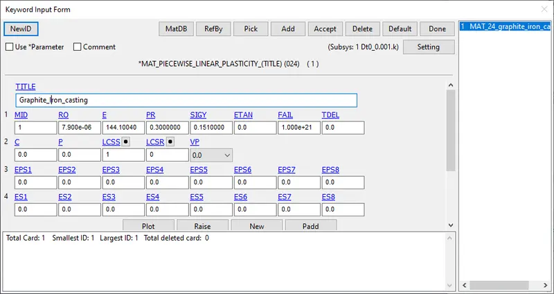
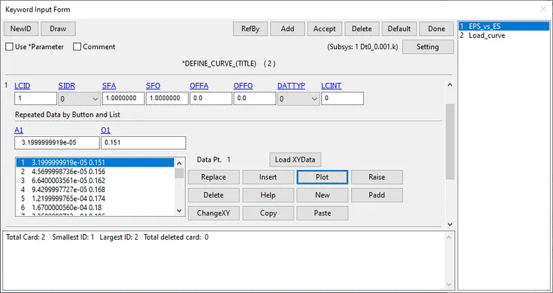
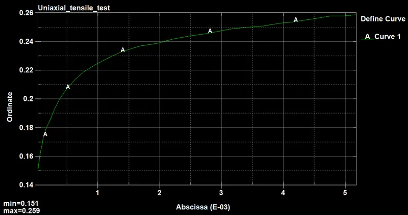
The LCSS contains the load curve of effective plastic strain EPS vs effective (true) stress ES.
The effective plastic strain is calculated in the excel sheet from the true stress value using the relation
Effective plastic strain = True strain - (True stress/ Young's modulus)
The region of the curve after the yield point (144 Gpa) is the plastic part of the curve. Therefore the values in the excel sheet after this stress point, and the corresponding EPS values are input into LS Dyna and the curve is generated as shown below.
Part definition
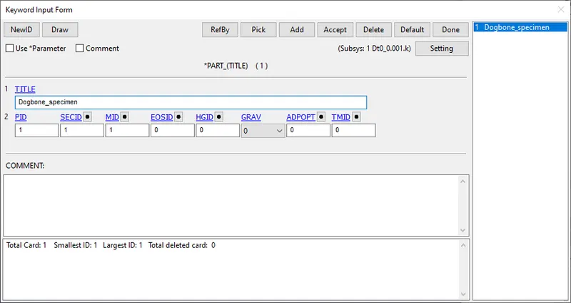
The material and the section ID are then assigned to the dogbone specimen part as shown below.
Step 3: Database and control cards
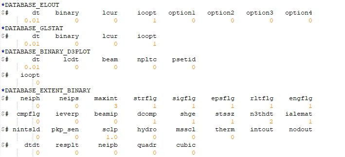
The database cards are defined as shown below.
The timestep for BINARY_D3PLOT and DATABASE_ASCII for GLSTAT and ELOUT are 0.1 ms.
DATABASE_EXTENT_BINARY card with STRFLG = 1 is used to compute the elastic strain in the model.
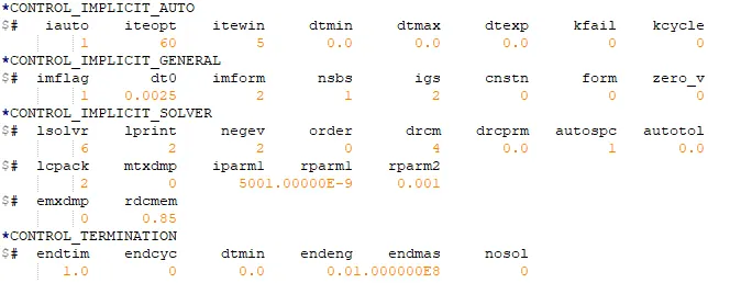
Since the tensile test of the specimen is a quasi-static analysis, it is carried out using an implicit scheme. The dt0 value is given as 0.0025 ms.
Results
The model is simulated and the results are discussed below.
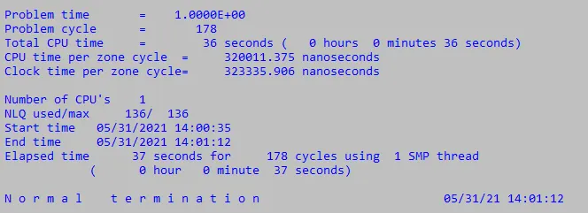
The animation of the von mises stress can be seen below.

The maximum stress is 0.2709 GPA, which is higher than the yield strength limit off 144 GPA. This means that plastic deformation occurs in the material. Necking, however, has not yet been develeoped.
The peak effective plastic strain is 0.00756.
The plots of X-stress and effective plastic strain of a particular element (330) in the middle of the specimen, are shown below.
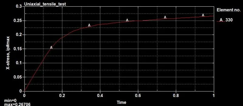
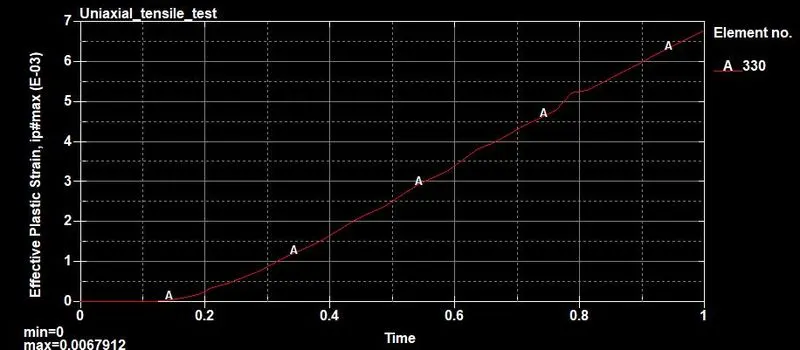
Using cross plot in LS Dyna, the values of true stress and strain can be plotted, as shown below.
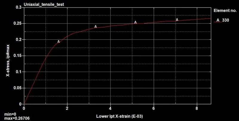
The stress and strain values can be exported into excel and compared with the plot from the raw data, to validate the results obtained.
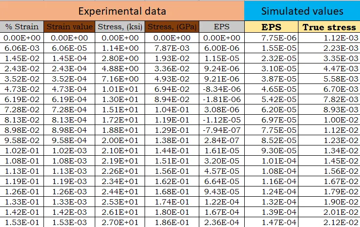
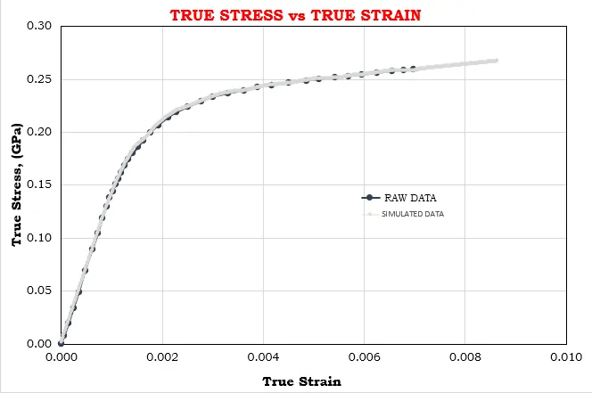
The curve exactly fits the experimental data. Therefore, the given values are validated using the MAT 24 card. In the simulation, the strain is higher than the experimental data (beyond 0.007), since the defined displacement causes a higher strain.
Conclusion
Thus the tensile test is performed on the given dogbone specimen and the simulated values of true stress and strain are validated with the experimental data.