Week 9 - FVM Literature Review

Objective :-

1. Define Finite Volume Method (FVM)

2. Diffrence between FDM &FVM

3. Describe Interploation Scheme.

4. Describe Flux Limiters.

1.Finite Volume Method (FVM)

Finite Volume Method with two Point of view i.e, Physical and Numerical Point of view.

From the physical point of view the FVM is based on balancing fluxes through control volumes, i. e. the Eulerian concept is used where the integral formulation of conservative laws are discretized directly in space.

From the numerical point of view the FVM is a generalization of the FDM in a geometric and topological sense, i. e. simple finite volume schemes can be reduced to finite difference schemes.

Advantages :

• It enforces conservation of quantities at discretized level, i. e. mass, momentum, energy remain conserved also at a local scale. Fluxes between adjacent control volumes are directly balanced.
• Finite volume schemes takes full advantage of arbitrary meshes to approximate complex geometries.

//////////////////////////////////////////////////////////////////////////////////////////////////////////////////////////////////////////

2.Diffrence Between Finite Diffrence Method(FDM) and Finite Volume Method(FVM)

Finite Diffrence Method (FDM) :

• A finite difference method (FDM) discretization is based upon the differential form of the PDE to be solved. Each derivative is replaced with an approximate difference formula (that can generally be derived from a Taylor series expansion).
• The computational domain is usually divided into hexahedral cells (the grid), and the solution will be obtained at each nodal point.
• The FDM is easiest to understand when the physical grid is Cartesian.
• The discretization results in a system of equation of the variable at nodal points, and once a solution is found, then we have a discrete representation of the solution.

Finite Volume Method (FVM) :

• A finite volume method (FVM) discretization is based upon an integral form of the PDE to be solved (e.g. conservation of mass, momentum, or energy).
• The PDE is written in a form which can be solved for a given finite volume (or cell).
• The computational domain is discretized into finite volumes and then for every volume the governing equations are solved. The resulting system of equations usually involves fluxes of the conserved variable, and thus the calculation of fluxes is very important in FVM.
• The basic advantage of this method over FDM is it does not require the use of structured grids, and the effort to convert the given mesh in to structured numerical grid internally is completely avoided.

///////////////////////////////////////////////////////////////////////////////////////////////////////////////////////////////////////////

3.Interploation Scheme in FVM :-

The approximation of surface and volume integrals may require values of the variables at locaion other than the computational nodes of the CV.Values are obtained using interpolation formulae.

CFD offer many diffrent types of Interpolation schemes :-

1. Upward
2. Liner (Central Diffrencing)
3. Linear Upward
4. Quadratic Upwind Interploation (QUICK)
5. Limited Linear

Now here we are going to interpolate a value of a gray face 'f' by taking an heat conduction, so to speak it's more of a face interpolation scheme.because we are interpolating using owner and neighbour cell.

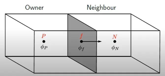
1. Linear/Central Diffrencing

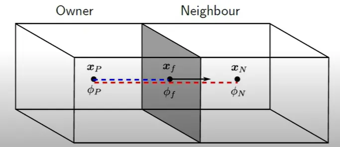
• ϕf=ψ.ϕN+(1−ψ)ϕP
• ψ=(xf−xp )/(xN−xp )
• 0≤ψ≤1
• This intepolation scheme is equivalent to the use of central Diffrencing formula of the first derivative.
• This scheme is second order accurate.
• But the scheme is unbounded.
• Example :- CDS is used for the diffusion term of NS eqaution.

2. Upward Diffrencing

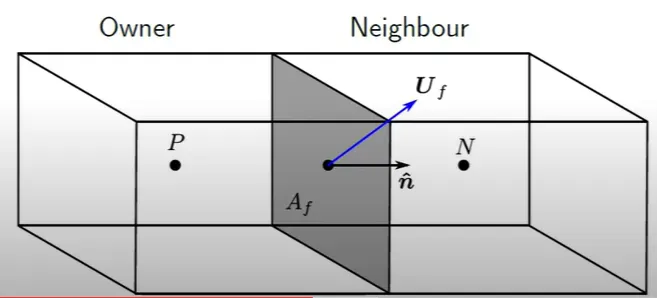
• Upward Diffrencing is depends on the direction of mass flux.

Ff=ρfAf(Uf.ˆn)

• Ff > 0 indicates mass flow out of the cell
• Ff <0 indicates mass flow into the cel
• 
• 
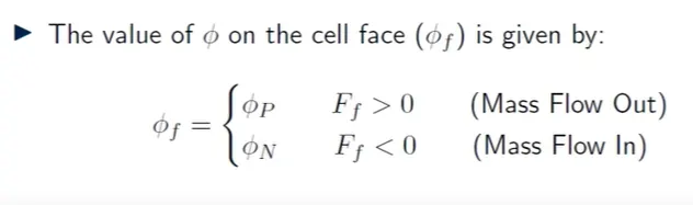
• This intepolation scheme is equivalent to the use of backward or forward finite diffrence approximation.
• Upwind is not accurate.
• But it is most stable for Convection dominated flow.
• We can use it generate an initial,stable solution,then we can use diffrent scheme.

//////////////////////////////////////////////////////////////////////////////////////////////////////////////////////////////////////////

4.Flux Limiters

Most of us might have seen the behaviour of numerical schemes in order to capture shocks and discontinuity that arises in hyperbolic equations. Physically, these equations model the convective fluid flow. It has been observed that low-order schemes are usually stable but quite dissipative in nature around the points of discontinuity/shocks. On the other hand higher-order numerical schemes are unstable in nature and show oscillations in the vicinity of discontinuity. One can have a better understanding of such behaviour by analysing the modified equation of these schemes.

Now as said above one can not have high order accuracy without oscillations. The objective is to have highly accurate and stable oscillation free schemes. This kind of schemes are known as high resolution schemes. In 1984 Harten proposed the constuction and gave TVD criteria for such scheme. Here we talk only about using flux limiters function to construct high resolution schemes.