Week 7 - Simulation of a 1D Super-sonic nozzle flow simulation using Macormack Method
Aim :- Simulation of a 1D Super-sonic nozzle flow simulation using Macormack Method
Objective :- To simulate the isentropic flow through a quasi 1D subsonic-supersonic nozzle,derive both the conservation and non-conservation forms of the governing equations .
You need to show the following plots inside your report
1. Steady-state distribution of primitive variables inside the nozzle
2. Time-wise variation of the primitive variables
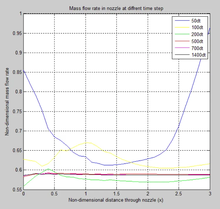
3. Variation of Mass flow rate distribution inside the nozzle at different time steps during the time-marching process
4. Comparison of Normalized mass flow rate distributions of both forms
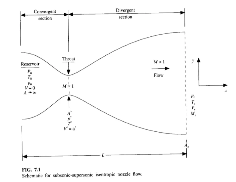
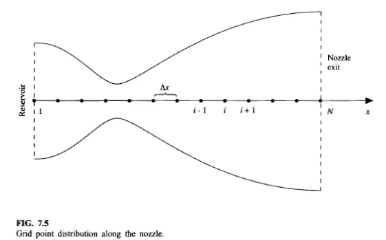
Diagram of subsonic-supersonic nozzle Flow :-
Macormack Technique :-
MacCormack's technique is a variant of the Lax-Wendroff approach but is much simpler in its application. Like the Lax-Wendroffmethod, the Maccormack method is also an explicit finite-difference technique which is second-order-accurate in both space and time.
MacCormack's technique is a two-step predictor-corrector sequence is used with forward differences on the predictor and with rearward differences on the corrector, is a second-order-accurate method.
In MacCormack's technique, the use of forward differences on the predictor and rearward differences on the corrector is not sacrosanct; the same order of accuracy is obtained by using rearward diffences on the predictor and forward differences on the corrector. Indeed, a time-marching solution can be carried out by altemating between these two sequences at every other time step, if you so choose.
Governing Equation :-
1. Non-Conservative Form :-
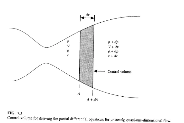
This control volume is a slice of the nozzle flow, where the infinitesimal thickness of the slice is dx. On the left side of the control volume, consistent with the quasi-one-dimensional assumption, the density, velocity, pressure, and internal energy, denoted by p,V, p, and e, respectively, are uniform over the area A.
1.Continuity Equation :-

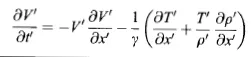
2.Momentum Equation :-
3.Energy Equation :-

Initial Conditions :-
Area of the Nozle :
`A=1+2.2(x−1.5)^2`
Density , Nozzle , Teperature of the nozzle :
`rho = 1 - 0.3146x`
`T = 1 -0.2314x`
`V = (0.1 + 1.09x)T^(1/2)`
Static ressure :-
`P = rho.T`
Mach Number :-
`M = V/(sqrtT)`
Boundary Conditions :-
By interpolating the variables :-
Subsonic inflow Boundary :
V1 = 2V2 - V3
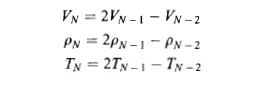
Supersonic outflow Boundary :
Discretization By Finite Diffrencing Method :-
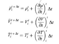
Macormack Techique :
1.Predictor Step
Continuity Equation

Momentum Equation

Energy Equation

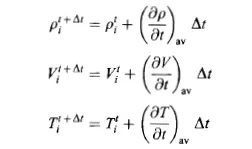
We obtain the predicted values of `rho`,T, & V,
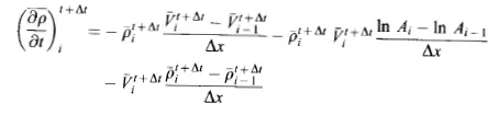
2.Predictor Step :
Continuity Equation
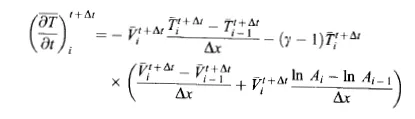
Momentum Equation

Energy Equation
The Average time Derivative are given by,
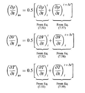
The Final values are :
2.Non-Conservation Form :-
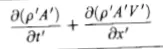
1.Continuity Equation :-
2.Momentum Equation :-

3.Energy Equation :-

Let us define the elements of the solutions vector U, the flux vector F, and the source term J as follows.
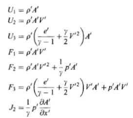
Now the Governing Equation can be written as,respectively,
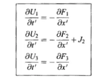
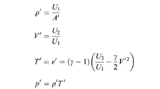
U is called the primitive variables,and to obtain the primitive vaiables we must decode U1,U2,U3 s follows,
"PURE" FORM OF THE FLUX TERMS
F1 = U2
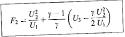
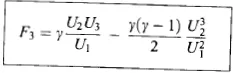
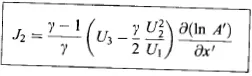
Sourcr term :
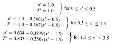
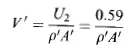
Initial Conditions :-
Boundary Conditions :-
By interpolating the variables :-
Subsonic inflow Boundary :

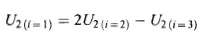
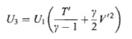
Supersonic outflow Boundary :
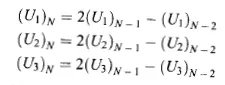
Similarly like Non-Conservation form, we will use the Macormack Technique to discretize it and after using the Predictor-Corrector step with forward differences on the predictor and with rearward differences on the corrector, is a second-order-accurate method, then the average time derivative values can be calculated by taking corrector and predictor time derivative values.
Calculating Time Step solution :
C is the Courant number,the simple stability analysis of a linear hyperbolic equation is C<=1.
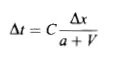
Minimum value of the time step is used to find the time derivative at each iteration:

Main Code :-
clear all
close all
clc

%inputs
n =31;
x = linspace(0,3,n);
dx = x(2)-x(1);
gamma = 1.4;
th = (n-1)/2 + 1;

A = 1 + 2.2*(x-1.5).^2;

%Non-Conservative Form
[dt,rho,t,v,~,mass_nc,mach_nc,P_nc,rhoth,Pth,vth,tth,massth] = Non_conservation_form(A,th,n,x,dx,gamma);

  figure(5)

   subplot(5,1,1)
   plot(x,rho)
   hold on;
   xlabel('Number of timesteps');
   ylabel('rho/rho_o');
   title('value at throat for variables timesteps');
    subplot(5,1,2);
   plot(x,t)
   hold on;
   xlabel('Number of timesteps');
   ylabel('T/T_o');
    subplot(5,1,3);
   plot(x,v)
   hold on;
   xlabel('Number of timesteps');
   ylabel('V/V_o');
    subplot(5,1,4);
   plot(x,P_nc)
   hold on;
   xlabel('Number of timesteps');
   ylabel('P/P_o');
    subplot(5,1,5)
   plot(x,mach_nc)
   hold on;
   xlabel('Number of timesteps');
   ylabel('mass flow rate');

%Conservative Form
[rhoc,tc,vc,nt,mass_c,mach_c,P_c,rhothc,Pthc,vthc,tthc,massthc,X]= Conservation_form(A,th,n,x,dx,gamma);

     figure(6)

   subplot(5,1,1)
   plot(x,rhoc)
   hold on;
   xlabel('Number of timesteps');
   ylabel('rho/rho_o');
   title('value at throat for variables timesteps');
    subplot(5,1,2);
   plot(x,tc)
   hold on;
   xlabel('Number of timesteps');
   ylabel('T/T_o');
    subplot(5,1,3);
   plot(x,vc)
   hold on;
   xlabel('Number of timesteps');
   ylabel('V/V_o');
    subplot(5,1,4);
   plot(x,P_c)
   hold on;
   xlabel('Number of timesteps');
   ylabel('P/P_o');
    subplot(5,1,5)
   plot(x,mach_c)
   hold on;
   xlabel('Number of timesteps');
   ylabel('mass flow rate');
Non-Conservation Form :-
function[dt,rho,t,v,nt,mass_nc,mach_nc,P_nc,rhoth,Pth,vth,tth,massth]=Non_conservation_form(A,th,n,x,dx,gamma)

%calculate the initial radius

t = 1-0.2314*x;
v = (0.1+1.09*x).*t.^0.5;
rho = 1-0.3146*x;

%time step
nt = 1400;
dt = 0.02;


%Outer time loop
for k=1:nt

    rho_old = rho;
    v_old = v;
    t_old = t;

    %predictor method
   for j = 2:n-1


    dvdx = (v(j+1)-v(j))/dx;
    drhodx = (rho(j+1)-rho(j))/dx;
    dtdx = (t(j+1)-t(j))/dx;
    dlogdx = (log(A(j+1))-log(A(j)))/dx;
    %continuity equation
    drhodt_p(j) = -rho(j)*dvdx-rho(j)*v(j)*dlogdx-v(j)*drhodx;
    %momentum equation
    dvdt_p(j) = -v(j)*dvdx-(dtdx+(drhodx*t(j)/rho(j)))/gamma;
    %energy equation
    dtdt_p(j) = -v(j)*dtdx-(gamma-1)*t(j)*(dvdx+v(j)*dlogdx);

    %solution update
    rho(j) = rho(j) + (drhodt_p(j)*dt);
    v(j) = v(j) + (dvdt_p(j)*dt);
    t(j) = t(j) + (dtdt_p(j)*dt);

   end


   %corrector method
   for j = 2:n-1


    dvdx = (v(j)-v(j-1))/dx;
    drhodx = (rho(j)-rho(j-1))/dx;
    dtdx = (t(j)-t(j-1))/dx;
    dlogdx = (log(A(j))-log(A(j-1)))/dx;
    %continuity equation
    drhodt_c(j) = -rho(j)*dvdx-rho(j)*v(j)*dlogdx-v(j)*drhodx;
    %momentum equation
    dvdt_c(j) = -v(j)*dvdx-(dtdx+(drhodx*t(j)/rho(j)))/gamma;
    %energy equation
    dtdt_c(j) = -v(j)*dtdx-(gamma-1)*t(j)*(dvdx+v(j)*dlogdx);

   end

   %Computing average derivative

   drhodt = 0.5*(drhodt_p+drhodt_c);
   dvdt = 0.5*(dvdt_p+dvdt_c);
   dtdt = 0.5*(dtdt_p+dtdt_c);

   %Final solution update

   for d = 2:n-1

       rho(d) = rho_old(d) + drhodt(d)*dt;
         v(d) = v_old(d) + dvdt(d)*dt;
         t(d) = t_old(d) + dtdt(d)*dt;
   end

   %Boundary Solution

   %Inlet BOundary Condition
   v(1) = 2*v(2) - v(3);

   %Outflow Boundary Condition
   rho(n) = 2*rho(n-1) - rho(n-2);
   v(n) = 2*v(n-1) - v(n-2);
   t(n) = 2*t(n-1) - t(n-2);

   %Mass flow rate
   mass_nc = rho.*A.*v;

   %Mach number
    mach_nc = v./(t.^0.5);

   %Pressure
   P_nc = rho.*t;


   figure(1);

   if j == 50
       plot(x,mass_nc,'b')
       hold on;
   elseif j == 100
       plot(x,mass_nc,'y')
   elseif j == 200
       plot(x,mass_nc,'g')
   elseif j == 500
       plot(x,mass_nc,'r')
   elseif j == 700
       plot(x,mass_nc,'m')
   elseif j == 1400
       plot(x,mass_nc,'k')
   xlabel('Non-dimensional distance through nozzle (x)')
   ylabel('Non-dimensional mass flow rate')
   title('Mass flow rate in nozzle at diffrent time step')
   legend('50dt','100dt','200dt','500dt','700dt','1400dt')
   grid on

   end


   %Field variables at throat section

   rhoth(k) = rho(th);
   tth(k) = t(th);
   vth(k) = v(th);
   Pth(k) = P_nc(th);
   massth(k) = mass_nc(th);

end


   figure(2)
   X = linspace(1,nt,nt);
   subplot(5,1,1)
   plot(X,rhoth)
   hold on;
   xlabel('Number of timesteps');
   ylabel('rho/rho_o');
   title('value at throat for variables timesteps');
    subplot(5,1,2);
   plot(X,tth)
   hold on;
   xlabel('Number of timesteps');
   ylabel('T/T_o');
    subplot(5,1,3);
   plot(X,vth)
   hold on;
   xlabel('Number of timesteps');
   ylabel('V/V_o');
    subplot(5,1,4);
   plot(X,Pth)
   hold on;
   xlabel('Number of timesteps');
   ylabel('P/P_o');
    subplot(5,1,5)
   plot(X,massth)
   hold on;
   xlabel('Number of timesteps');
   ylabel('mass flow rate');


end
Conservation Form :-
function[rhoc,tc,vc,nt,mass_c,mach_c,P_c,rhothc,Pthc,vthc,tthc,massthc,X]= Conservation_form(A,th,n,x,dx,gamma)

%Initial Condition
for i=1:n
    if (x(i)>=0) && (x(i)<0.5)
        rhoc(i) = 1;
        tc(i)=1;
    elseif (x(i)>=0.5) && (x(i)<1.5)
        rhoc(i) = 1 - 0.366*(x(i)-0.5);
        tc(i) = 1 - 0.167*(x(i)-0.5);
    elseif (x(i)>=1.5) && (x(i)<3.5)
        rhoc(i) = 0.634 - 0.3879*(x(i)-1.5);
        tc(i) = 0.833 - 0.3507*(x(i)-1.5);
    end
end

%Velocity
vc = (0.59)./(rhoc.*A);

nt =1400;
U1 = rhoc.*A;
U2 = rhoc.*A.*vc;
U3 = rhoc.*A.*((tc./(gamma-1))+(gamma/2).*(vc.^2));


for k =1:n
    dt_c(k) = (0.5*dx)/((sqrt(tc(i)))+vc(k));
end

dt = min(dt_c);

%Outer time loop
for j = 1:nt
    U1_old = U1;
    U2_old = U2;
    U3_old = U3;


    %Flux terms
    F1 = U2;
    F2 = (((U2.^2)./U1)+((gamma-1)/gamma)*(U3-(gamma/2)*((U2.^2)./U1)));
    F3 = ((gamma.*U2.*U3)./U1)-((gamma/2)*(gamma-1).*((U2.^3)./(U1.^2)));

    %predictor method

    for i = 2:n-1

        %Continuity equation
        dU1dt_p(i) = -((F1(i+1)-F1(i))/dx);

        %Momentum Equation
        J2(i) = ((gamma-1)/gamma)*(U3(i)-(gamma/2)*((U2(i).^2)/U1(i)))*(((log(A(i+1))-log(A(i)))/dx));
        dU2dt_p(i) = -(((F2(i+1)-F2(i))/dx))+J2(i);

        %Energy Equation
        dU3dt_p(i) = -((F3(i+1)-F3(i))/dx);


        %solution update
        U1(i) = U1(i) + dU1dt_p(i)*dt;
        U2(i) = U2(i) + dU2dt_p(i)*dt;
        U3(i) = U3(i) + dU3dt_p(i)*dt;

    end


    rhoc = U1./A;
    vc = (U2./(U1));
    tc = (gamma-1)*((U3./U1)-((gamma/2)*(vc.^2)));

    %Flux terms
    F1 = U2;
    F2 = ((U2.^2)./U1)+((gamma-1)/gamma)*(U3-(gamma/2)*((U2.^2)./U1));
    F3 = ((gamma.*U2.*U3)./U1)-((gamma/2)*(gamma-1).*((U2.^3)./(U1.^2)));

    %corrector method
    for i = 2:n-1

        %Continuity equation
        dU1dt_c(i) = -((F1(i)-F1(i-1))/dx);

        %Momentum Equation
         J2(i) = ((gamma-1)/gamma)*(U3(i)-(gamma/2)*((U2(i).^2)/U1(i)))*(((log(A(i))-log(A(i-1)))/dx));
         dU2dt_c(i) = -(((F2(i)-F2(i-1))/dx))+J2(i);


        %Energy Equation
        dU3dt_c(i) = -((F3(i)-F3(i-1))/dx);

    end
     %Computing average derivative

       dU1dt = 0.5*(dU1dt_p + dU1dt_c);
       dU2dt = 0.5*(dU2dt_p + dU2dt_c);
       dU3dt = 0.5*(dU3dt_p + dU3dt_c);


   for k = 2:n-1

       U1(k) = U1_old(k) + dU1dt(k)*dt;
       U2(k) = U2_old(k) + dU2dt(k)*dt;
       U3(k) = U3_old(k) + dU3dt(k)*dt;
   end

      %Boundary Solution

   %Inlet BOundary Condition
   U1(1) = rhoc(1)*A(1);
   U2(1) = 2*U2(2)-U2(3);
   U3(1) = U1(1)*((tc(1)./(gamma-1)) + ((gamma/2)*vc(1).^2));

   %Outflow Boundary Condition
   U1(n) = 2*U1(n-1) - U1(n-2);
   U2(n) = 2*U2(n-1) - U2(n-2);
   U3(n) = 2*U3(n-1) - U3(n-2);


  rhoc = U1./A;
    vc = U2./(U1);
    tc = (gamma-1)*((U3./U1)-((gamma/2).*(vc.^2)));

 %Mass flow rate
   mass_c = rhoc.*A.*vc;

   %Mach number
   mach_c = vc./(tc.^0.5);

   %Pressure
   P_c = rhoc.*tc;


   figure(3);

   if j == 50
       plot(x,mass_c,'b')
       hold on;
   elseif j == 100
       plot(x,mass_c,'y')
   elseif j == 200
       plot(x,mass_c,'g')
   elseif j == 500
       plot(x,mass_c,'r')
   elseif j == 700
       plot(x,mass_c,'m')
   elseif j == 1400
       plot(x,mass_c,'k')
   xlabel('Non-dimensional distance through nozzle (x)')
   ylabel('Non-dimensional mass flow rate')
   title('Mass flow rate in nozzle at diffrent time step')
   legend('50dt','100dt','200dt','500dt','700dt','1400dt')
   grid on

   end

   %Field variables at throat section

   rhothc(j) = rhoc(th);
   tthc(j) = tc(th);
   vthc(j) = vc(th);
   Pthc(j) = P_c(th);
   massthc(j) = mass_c(th);

end


   figure(4)
   X = linspace(1,nt,nt);
   subplot(5,1,1)
   plot(X,rhothc)
   hold on;
   xlabel('Number of timesteps');
   ylabel('rho/rho_o');
   title('value at throat for variables timesteps');
   subplot(5,1,2);
   plot(X,tthc)
   hold on;
   xlabel('Number of timesteps');
   ylabel('T/T_o');
   subplot(5,1,3);
   plot(X,vthc)
   hold on;
   xlabel('Number of timesteps');
   ylabel('V/V_o');
   subplot(5,1,4);
   plot(X,Pthc)
   hold on;
   xlabel('Number of timesteps');
   ylabel('P/P_o');
   subplot(5,1,5)
   plot(X,massthc)
   hold on;
   xlabel('Number of timesteps');
   ylabel('mass flow rate');


end
Mass Flow rate at diffrent time step :-
Conservation Form :-
Value at throat at variable timestep
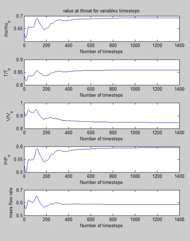
Timewise variations of the density, temperature, pressure, and Mach number at the nozzle throat :-
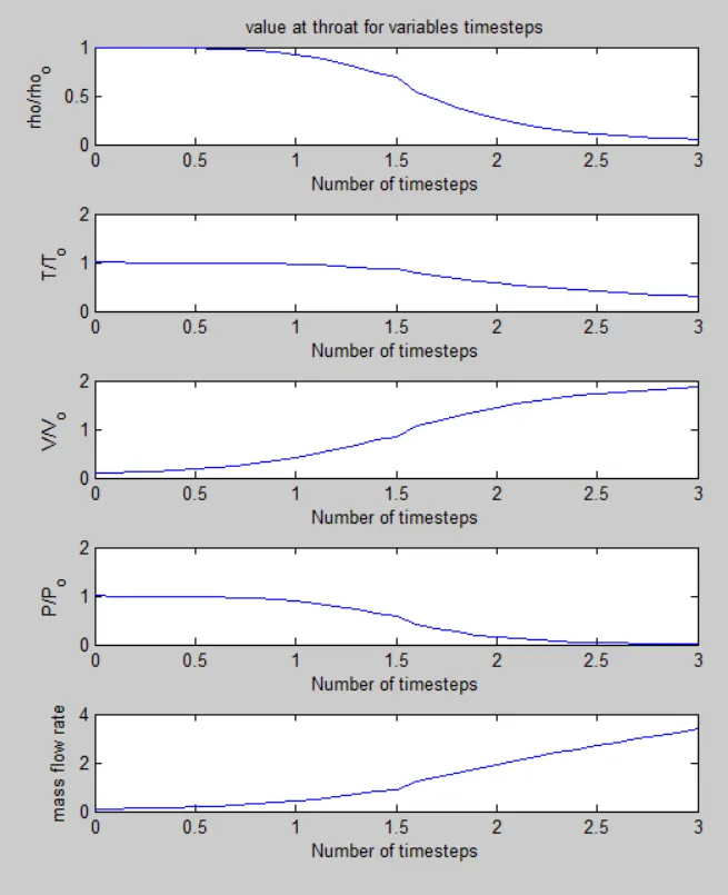
Non-Conservation :-
Value at throat at variable timestep
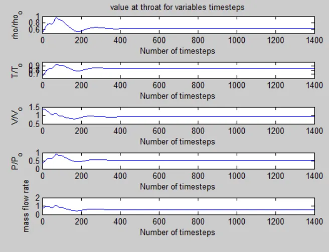
Timewise variations of the density, temperature, pressure, and Mach number at the nozzle throat :-
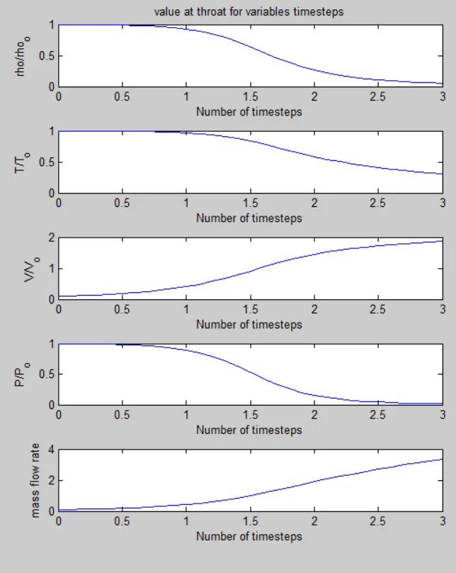
Conclusion :-
From the graphs and tables we can conslude that Non conservation is more precised in away compared to Conservation form.
Referance :-
John Anderson Jr. Book
NPTEL CFD by Suman Chakraborty