Challenge

Week 9 - FVM Literature Review

JJaswanth Sai Padugupadu7 Oct 2024

Finite Volume Method (FVM) Overview

The Finite Volume Method (FVM) is a numerical technique used for solving partial differential equations (PDEs), particularly those that arise in fluid dynamics, heat transfer, and other engineering fields. FVM is based on the conservation principle, and its key advantage is that it ensures the conservation of quantities such as mass, momentum, or energy at the control volume level.

In FVM, the computational domain is divided into small control volumes (CVs). The governing equation is integrated over each CV, and fluxes are calculated across the CV boundaries. The flux balance within each CV determines the values of the dependent variables.

Key Steps in FVM:

Divide the domain into control volumes.
Integrate the governing equation over each control volume.
Apply boundary and initial conditions.
Approximate the surface fluxes and gradients using interpolation or other schemes.
Solve the resulting algebraic equations for the unknowns.

1D Linear Heat Conduction Equation Example

Consider the 1D linear heat conduction equation:

$\frac{\partial T}{\partial t} = \alpha \frac{\partial^2 T}{\partial x^2}$

where:

$T$ is the temperature,
$\alpha$ is the thermal diffusivity,
$x$ is the spatial coordinate,
$t$ is time.

In FVM, the equation is discretized by integrating over each control volume.

Finite Difference Method (FDM) vs. Finite Volume Method (FVM)

Major Differences:

Aspect	Finite Difference Method (FDM)	Finite Volume Method (FVM)
Approach	Solves PDEs by approximating derivatives at discrete points.	Solves PDEs by integrating over control volumes.
Conservation	Not inherently conservative.	Conservative by design, ensures local and global conservation.
Mesh Flexibility	Structured, usually requires regular grids.	Can handle structured and unstructured meshes.
Flux Calculation	No direct calculation of fluxes.	Fluxes are explicitly calculated across control volume faces.
Geometry Handling	Difficult to handle complex geometries.	Suitable for complex geometries due to control volume flexibility.
Boundary Conditions	Directly applied at grid points.	Applied to control volume surfaces.

Need for Interpolation Schemes in FVM

In FVM, interpolation schemes are necessary to estimate the values of variables at control volume faces (midpoints between grid points) since the values are known only at the centroids of control volumes. These schemes help in calculating fluxes across the faces of the control volumes. Common interpolation schemes include:

Central Differencing Scheme (CDS):
- A simple averaging scheme, used for linear problems but may introduce oscillations in convection-dominated flows.
- For 1D, temperature at face $T_f$ is interpolated as:
Tf=TP+TE2T_f = \frac{T_P + T_E}{2}
where $T_P$ and $T_E$ are the temperatures at the neighboring control volume centers.
Upwind Scheme:
- Based on the flow direction; more stable for convection-dominated problems.
- For 1D, if the flow is from left to right:
Tf=TPT_f = T_P
where $T_P$ is the upstream value (control volume on the left).
Linear Upwind Scheme:
- Higher-order approximation that takes into account the variation within the control volume.

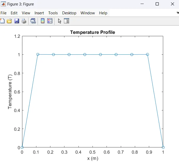
MATLAB Code: Interpolation for 1D Heat Conduction:

% Parameters

L = 1; % Length of the rod (m)

Nx = 10; % Number of control volumes

dx = L / Nx; % Control volume size

alpha = 1e-5; % Thermal diffusivity (m^2/s)

dt = 0.01; % Time step (s)

nt = 100; % Number of time steps

% Initial temperature profile (1D array for temperature at CV centers)

T = ones(Nx, 1); % Initial temperature = 1 everywhere

% Boundary conditions

T_left = 0; % Left boundary temperature

T_right = 0; % Right boundary temperature

% Time-stepping loop

for n = 1:nt

% Compute fluxes at CV faces using Central Differencing Scheme (CDS)

for i = 2:Nx-1

T_face_left = (T(i-1) + T(i)) / 2; % Interpolated value at left face

T_face_right = (T(i) + T(i+1)) / 2; % Interpolated value at right face

% Discretized 1D heat conduction equation

flux_left = alpha * (T(i) - T(i-1)) / dx;

flux_right = alpha * (T(i+1) - T(i)) / dx;

% Update temperature at the current control volume

T(i) = T(i) + dt * (flux_left - flux_right) / dx;

end

% Apply boundary conditions

T(1) = T_left;

T(Nx) = T_right;

end

% Plot the final temperature profile

x = linspace(0, L, Nx);

plot(x, T, '-o');

xlabel('x (m)');

ylabel('Temperature (T)');

title('Temperature Profile');

Flux Limiters in FVM

Flux limiters are used in conjunction with higher-order schemes to prevent numerical oscillations (such as overshoots or undershoots) in the solution, especially in convection-dominated problems. They blend between low-order and high-order schemes depending on the local smoothness of the solution, providing the best balance between accuracy and stability.

Low-order schemes (like upwind) are stable but introduce numerical diffusion.
High-order schemes (like central differencing) are accurate but can introduce oscillations.
Flux limiters help in choosing an optimal combination to maintain stability and accuracy.

A commonly used flux limiter is the van Leer limiter.

Week 9 - FVM Literature Review

Finite Volume Method (FVM) Overview

Key Steps in FVM:

1D Linear Heat Conduction Equation Example

Finite Difference Method (FDM) vs. Finite Volume Method (FVM)

Major Differences:

Need for Interpolation Schemes in FVM

Flux Limiters in FVM

Ship work like this
in your own course.

Talk to a career counsellor

Finite Volume Method (FVM) Overview

Key Steps in FVM:

1D Linear Heat Conduction Equation Example

Finite Difference Method (FDM) vs. Finite Volume Method (FVM)

Major Differences:

Need for Interpolation Schemes in FVM

Flux Limiters in FVM

Ship work like thisin your own course.

Talk to a career counsellor

Ship work like this
in your own course.