Week 9 - FVM Literature Review
AIM: To understand about finite volume method, the basic difference between the other methods of discretization and to describe the various interpolation schemes. Also to learn about flux limiters.
Types of Discretization methods used in CFD:
- Finite Volume Method
- Finite Difference Method
- Finite Element Method
What is Finite Volume Method?
The finite volume method (FVM) is a method for representing and evaluating partial differential equations in the form of algebraic equations. In the finite volume method, volume integrals in a partial differential equation that contain a divergence term are converted to surface integrals, using the divergence theorem. These terms are then evaluated as fluxes at the surfaces of each finite volume. Because the flux entering a given volume is identical to that leaving the adjacent volume, these methods are conservative. Another advantage of the finite volume method is that it is easily formulated to allow for unstructured meshes.
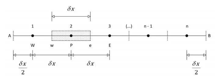
Let us cosider the 1D convection equation.
`d/dx(Gamma (d phi)/(dx))+S=0`
where Γ is the diffusion coefficient and S is the source term.
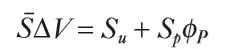
Now in order to invoke the FVM we integrate the above equation over a controled volume which on further solving gives us the discretised equation at point p as in figure.

The above equation is solved to yield the following.

Interpolating Schemes
There are a few types of interpolation schemes which are mentioned below:
- Upwind Interpolation
- Linear Interpolation
- QUICK Interpolation
- Hybrid Scheme
- Total Variation Diminish
Upwind Interpolation
This scheme is based on direction of flow of the velocity. Here the node that lies in the upstream is considered for discretisation, thus the name. By this method we can calculate the values of flux on the east or the west side. This is dependant on the convention we choose. If we consider positive flow, it flows from west to east and vice versa is negative.
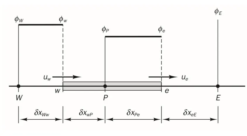
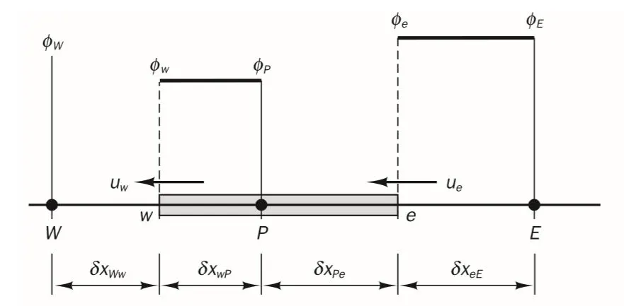
As mentioned above the flow of velocity is from west to east which signifies positive flow. Similarly for negative, the figure is given below:
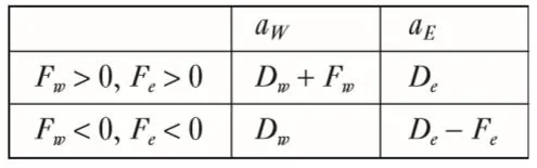
When the flow is in the positive direction, `u_w `> 0, `u_e` > 0 (`F_w` > 0,` F_e `> 0), the upwind scheme sets
`phi_w=phi_W` and `phi_e= phi_E`
The discretised form is given below:

When the flow is in the negative direction, `u_w` < 0, `u_e` < 0 (`F_w` < 0, `F_e` < 0), the scheme takes
`phi_w=phi_W` and `phi_e= phi_E`
The discretised form is given below:

Linear Interpolation
Approximates `phi_e` (value at face center) by its linear interpolation between two nearest nodes:

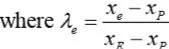
This scheme is also called central differencing scheme.
QUICK Interpolation
The quadratic upstream interpolation for convective kinetics (QUICK) scheme uses a three-point upstream-weighted quadratic interpolation for cell face values. The face value of φ is obtained from a quadratic function passing through two bracketing nodes (on each side of the face) and a node on the upstream side.

Coefficients in terms of nodal coordinates:
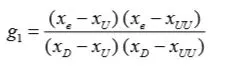
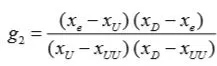
Approximation is 3nd order accurate on both uniform and non-uniform grids. For uniform grids:

Hybrid Scheme
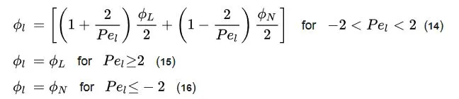
The hybrid differencing scheme of is based on a combination of central and upwind differencing schemes. The hybrid differencing scheme uses piecewise formulae based on the local Peclet number to evaluate the net flux through each control volume face. The Peclet number is evaluated at the face of the control volume.
Flux Limiters:
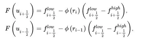
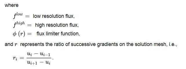
Flux limiters are used in high resolution schemes – numerical schemes used to solve problems in science and engineering, particularly fluid dynamics, described by partial differential equations (PDE's). They are used in high resolution schemes, such as the MUSCL scheme, to avoid oscillations that would otherwise occur with high order spatial discretization schemes due to shocks, discontinuities or sharp changes in the solution domain.
The main idea behind the construction of flux limiter schemes is to limit the spatial derivatives to realistic values – for scientific and engineering problems this usually means physically realisable and meaningful values. They are used in high resolution schemes for solving problems described by PDEs and only come into operation when sharp wave fronts are present. For smoothly changing waves, the flux limiters do not operate and the spatial derivatives can be represented by higher order approximations without introducing spurious oscillations.
References:
https://en.wikipedia.org/wiki/Flux_limiter
https://en.wikipedia.org/wiki/Hybrid_difference_scheme
An Introduction to Computational Fluid Dynamics
THE FINITE VOLUME METHOD
Second Edition
H K Versteeg and W Malalasekera