Understanding Linear Systems
AIM: To understand the convergence in matrix by finding the iterative matrix utilizing iterative solvers. Also to understand the importance of spectral radius for convergence.
HOW ARE EIGEN VALUES CALCULATED?
The genearal equation used to calculate the eigen values is as follows:
`abs(A-lambdaI)=0`
Where, `lambda` denotes the eigen values. The spectral radius denoted by `rho` is the maximum.
For a 3x3 matrix, the characteristic equation given below is used to evaluate the eigen values:
`lambda^3 +A lambda^2 +B lambda +C`
Where, `lambda` is the Eigen value,
A is the trace of the transformation matrix,
B is the sum of minors of the diagonal elements
C is the determinant of the transformation matrix.
However, the above is represented as below in order to evaluate the values of the same in the code.
`CP=−λ^3+tr(A)λ^2+0.5*(tr(A)^2−tr(A^2))λ+det(A)`
UNDERSTANDING CONVERGENCE IN MATRICES
The given matrix was `A=[[5,1, 2] ,[-3, 9, 4], [1, 2, -7]]` and `B=[(10),(-14),( 33)]`. If we look for the spectral radius of this matrix, it is higher than 1 (ie. 5.4569).
So, convergence in a matrix can be studied only on a iteration matrix. In order to implement the same, we use the common types of solvers.
- Jocobi Method
- Gauss Siedel Method
- Successive Over Relaxation Method
The following are the formulae to implement the iteration matrices using the above method:
Jocobi Method
Iterative matrix=`D^(-1)(L+U)`
Gauss Siedel Method
Iterative Matrix=`(D+L)^(-1)*U`
Successive Over Relaxation Method
Iterative Matrix=`(D+omega*L)^(-1)*(omega*U+(1-omega)*D)`
Where ,
D is the diagonal matrix, L is the lower triangular matrix, and U is the upper triangular matrix
MAIN CODE:
##A=[5 1 2 ; -3 9 4; 1 2 -7]
##
##X=[x1;x2;x3]
##
##B=[10 -14 33]
##
##Determine
##
##    Eigen values of iteration matrix.
##    Spectral radius of iteration matrix.
##    Solve the system using Jacobi, Gauss-seidel and SOR methods
##    Compute the iteration Matrix for the above mentioned iterative methods.
##    Increase the Spectral radius to 1.1 by changing the diagonal terms suitably.

 clear all
 close all
 clc

 A=[5 1 2 ; -3 9 4; 1 2 -7];
 %X=[x1;x2;x3]
 B=[10; -14; 33];

 % Separating into lower,upper triangle followed by the diagonal matrix

 D=diag(diag(A));
 L=tril(A)-D;
 U=triu(A)-D;
 eigen_cal= [-1,trace(A),0.5*(trace(A)^2-trace(A^2)),det(A)]; % coefficients of the characteristic equation
 eigen_val=roots(eigen_cal);
 spectral_rad_A=max(abs(real(eigen_val)));

 m=[0.46,0.5,1,2,3,4,6];
 %m=1;
 w=0.8
 %eig_jac_val=[];
 %eig_GS_val=[];
 %eig_SOR_val=[];

for i=1:length(m)
    d=m(i)*D;
    %d=D;
    I_jac=inv(d)*(L+U);

    %eigen value for the iteration matrix
    eig_jac=[-1 trace(I_jac) 0.5*(trace(I_jac)^2-trace(I_jac^2)) det(I_jac)];
    k= roots(eig_jac);
    spectral_rad_jac(i)=max(abs(real(k)));


    I_GS=(inv(d+L))*U;

    %eigen value for the iteration matrix
    eig_GS=[-1 trace(I_GS) 0.5*(trace(I_GS)^2-trace(I_GS^2)) det(I_GS)];
    r=roots(eig_GS);
    spectral_rad_GS(i)=max(abs(real(r)));

    I_SOR=(inv(d+(w*L)))*(w*U+(1-w)*d);

    %eigen value for the iteration matrix
    eig_SOR=[-1 trace(I_SOR) 0.5*(trace(I_SOR)^2-trace(I_SOR^2)) det(I_SOR)];
    e=roots(eig_SOR);
    spectral_rad_SOR(i)=max(abs(real(e)));

    %jocobi
    if spectral_rad_jac(i)<1
      [jac_iter(i),x]=jocobi_spec(A,B,d,L,U,m,I_jac);
      fprintf("n Jocobi methodn")
      fprintf("n spectral radius =%f n number iteration=%dn",spectral_rad_jac(i),jac_iter(i))
    else
      jac_iter(i)=nan;
      fprintf("n The solution is unstable for a magnification factor=%f and spec_jac=%fn",m(i),spectral_rad_jac(i))
     end

 %M_jac=jocobi_spec(A,B,D,L,U,m)

 %GS
    if spectral_rad_GS(i)<1
      [GS_iter(i),y]=GS_spec(A,B,d,L,U,m,I_GS);
      fprintf("n GS methodn")
      fprintf("n spectral radius =%f n number iteration=%dn",spectral_rad_GS(i),GS_iter(i))

    else
      GS_iter(i)= nan;
      fprintf("n The solution is unstable for a magnification factor=%f and spec_GS=%fn",m(i),spectral_rad_GS(i))
    end
 %SOR
    if spectral_rad_SOR(i)<1
      [SOR_iter(i),z] =SOR_spec(A,B,d,L,U,m,I_SOR);
      fprintf("n SOR methodn")
      fprintf("n spectral radius =%f n number iteration=%dn",spectral_rad_SOR(i),SOR_iter(i))

    else
      SOR_iter(i)=nan;
      fprintf("n The solution is unstable for a magnification factor=%f and spec_SOR=%fn",m(i),spectral_rad_SOR(i))

    end
end

  figure(1)
  subplot(3,1,1)
  plot(m,spectral_rad_jac,'-rx','linewidth',3,'markerfacecolor','k','markeredgecolor','k')
  xlabel("magnification factor");
  ylabel("spectral radius")
  title("Jocobi method","fontsize",15);
  grid on

  subplot(3,1,2)
  plot(m,jac_iter,'-bx','linewidth',3,'markerfacecolor','r','markeredgecolor','r')
  xlabel("magnification factor");
  ylabel("number of iteration")
  grid on

  subplot(3,1,3)
  plot(spectral_rad_jac,jac_iter,'-cx','linewidth',3,'markerfacecolor','g','markeredgecolor','g')
  xlabel("spectral radius");
  ylabel("number of iteration")
  grid on

  figure(2)
  subplot(3,1,1)
  plot(m,spectral_rad_GS,'-rx','linewidth',3','markerfacecolor','k','markeredgecolor','k')
  xlabel("magnification factor");
  ylabel("spectral radius")
  title("GS method","fontsize",15);
  grid on

  subplot(3,1,2)
  plot(m,GS_iter,'-bx','linewidth',3,'markerfacecolor','r','markeredgecolor','r')
  xlabel("magnification factor");
  ylabel("number of iteration")
  grid on

  subplot(3,1,3)
  plot(spectral_rad_GS,jac_iter,'-cx','linewidth',3,'markerfacecolor','g','markeredgecolor','g')
  xlabel("spectral radius");
  ylabel("number of iteration")
  grid on

  figure(3)
  subplot(3,1,1)
  plot(m,spectral_rad_SOR,'-rx','linewidth',3,'markerfacecolor','k','markeredgecolor','k')
  xlabel("magnification factor");
  ylabel("spectral radius")
  title("SOR method","fontsize",15);
  grid on

  subplot(3,1,2)
  plot(m,SOR_iter,'-bx','linewidth',3,'markerfacecolor','r','markeredgecolor','r')
  xlabel("magnification factor");
  ylabel("number of iteration")
  grid on

  subplot(3,1,3)
  plot(spectral_rad_SOR,jac_iter,'-cx','linewidth',3,'markerfacecolor','g','markeredgecolor','g')
  xlabel("spectral radius");
  ylabel("number of iteration")
  grid on


JOCOBI METHOD
 %jocobi method for matrix
 function [jac_iter, x]=jocobi_spec(A,B,d,L,U,m,I_jac)

  xold = [0;0;0];
  error=9e9;
  tol=1e-4;
  jac_iter=1;

    while (error>tol)
      x=(inv(d)*B)-(I_jac*xold);
      error= max(abs(xold-x));
      xold=x;
      jac_iter=jac_iter+1;
    end


 endfunction

GAUSS SIEDEL METHOD
  %GS method for matrix
 function [GS_iter,y]=GS_spec(A,B,d,L,U,m,I_GS)
  y=zeros(3,1);
  yold=y;

  error=9e9;
  tol=1e-4;
  GS_iter=1;


    while (error>tol)
      y=inv(d+L)*B-I_GS*yold;
      error=max(max(abs(yold-y)));
      yold=y;
      GS_iter=GS_iter+1;
    end


 endfunction

SOR METHOD:
 %SOR method for matrix
 function [SOR_iter,z]=SOR_spec(A,B,d,L,U,m,I_SOR)
  z=zeros(3,1);
  zold=z;

  error=9e9;
  tol=1e-4;
  SOR_iter=1;
  w=0.8;

      while (error>tol)
      z=I_SOR*zold+(inv(d+(w*L))*B);
      error=max(max(abs(zold-z)));
      zold=z;
      SOR_iter=SOR_iter+1;
    end


 endfunction
RESULTS:
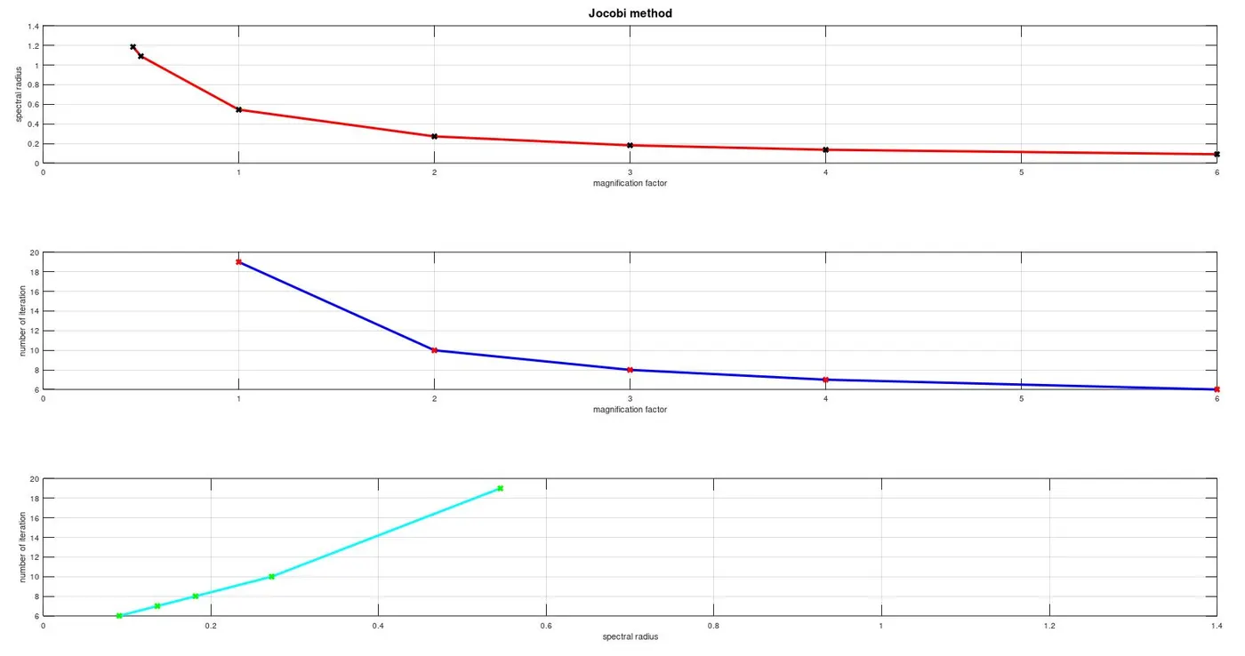
Jocobi method:
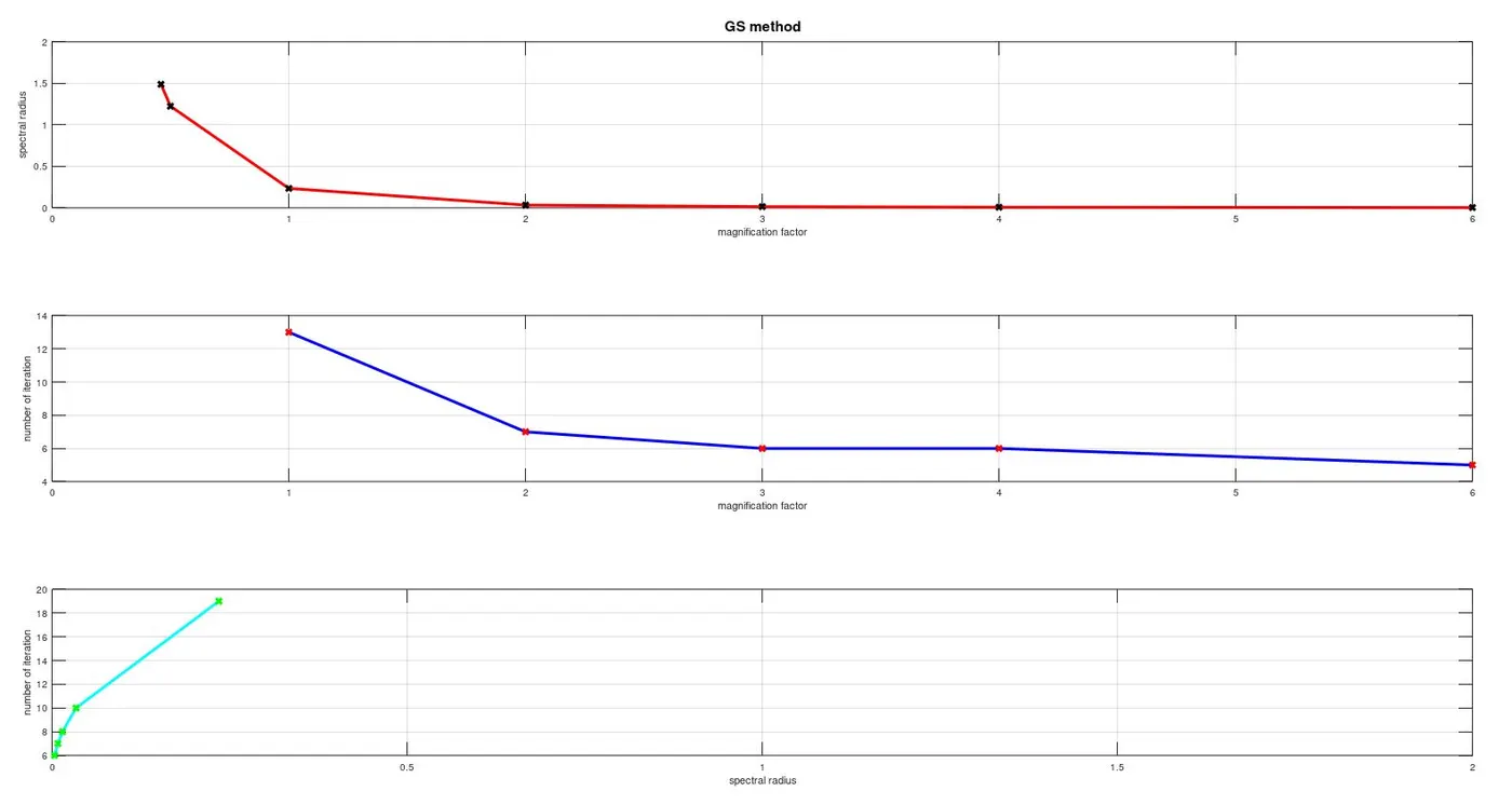
Gauss Siedel Method:
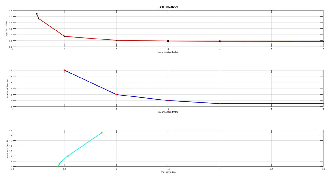
SOR Method:
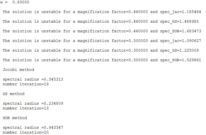
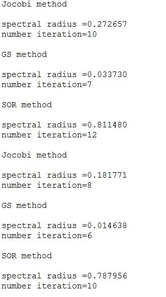
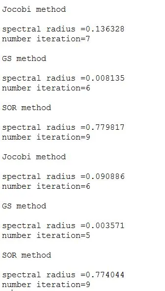
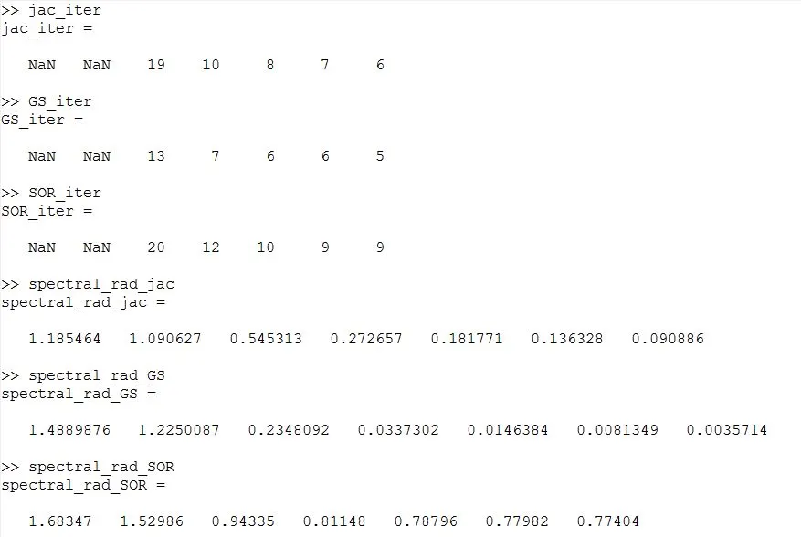
Output From the Command Screen:
INFERENCE:
- By this challenge we can infer the importance of diagonal dominance in order for the solution to converge
- When we increase the value of the diagonal elements by introducing a magnification factor, it was observed that the solution converged sooner for higher values of the magnification factor.
- Thus we can infer that the more dominant the diagonal elements are the less is the spectral radius and thus higher convergence.
- When the value of the spectral radius `rho`>1 the solution dosen't converge in any of the cases.