Solving the 2D Steady and Unsteady State Conduction Equation Using Octave
What is conduction?
Conduction is a method of heat transfer in which the transfer of energy takes place as a result of interactions between particles of higher energy and the particles of lower energy. The mode of energy transfer is particle collisions or lattice viberation dependant on the mediumin which the heat is being transfered.
In simple terms we could define conduction as the heat transfer taking place between a object with higher temperature and another object of lower temperature by contact.
STEADY STATE CONDITION
The 2 dimentional heat equation is given as follows:
`(delT)/(delt)+alpha((del^2T)/(delx^2)+(del^2T)/(dely^2))=0`
The above equation is the transient state equation. Below is the equation in steady state.
`(del^2T)/(delx^2)+(del^2T)/(dely^2)=0`
The above equation could also be written as,
`gradT=0`
The above equation is discretized using the central scheme as the above is a second order PDE and its solution would be elliptic.
In x direction:
`(del^2T)/(delx^2)=(T_L-2T_p+T_R)/(Deltax^2)`
In y direction:
`(del^2T)/(dely^2)=(T_T-2T_p+T_B)/(Deltay^2)`
The discretized form is given below:
`(T_L-2T_p+T_R)/(Deltax^2) +(T_T-2T_p+T_B)/(Deltay^2)=0`
Since we assume that nx=ny (ie. number of grid points=10) henct the above equation changes to the following:
`T_p=((T_L+T_R) +(T_T+T_B))/4`
CODE FOR STEADY STATE CONDUCTION:
Main Code:
 % 2D steady and unsteady problem
 % domain is a unit square
 % nx=ny
 %boundary Conditions for steady and transient
 %T_left=400k
 %T_top=600k
 %T_right=800k
 %T_bottom=900k

 %*******************Steady State******************************

 % d^2T/dx^2 +d^2T/dy^2=0
 clear all
 close all
 clc

 L=1;
 nx=10;
 ny=nx;
 x=linspace(0,L,nx);
 dx=x(2)-x(1);
 y=linspace(0,L,ny);
 dy=y(2)-y(1);

 % Setting the initial conditions
 T= ones(nx,ny)*298;

 T(:,1)=400; %left temp
 T(:,end)=800; %right temp
 T(end,:)=600; %top1 temp
 T(1,:)=900; %bottom temp

 % setting temperatures at either endswitch
 T(1,1)=(400+600)/2;
 T(nx,ny)=(800+900)/2;
 T(1,ny)=(600+800)/2;
 T(nx,1)=(400+900)/2;

 %Creating a copyfile
 Told=T;
 Tini=Told;
 error=9e9;
 tol=1e-4;
 [X,Y]=meshgrid(x,y);

 % we consider a variable iter_sol to invoke the different methods of iterative solvers
 %iter_sol=1 jocobi
 %iter_sol=2 G.S
 %iter_sol=3 SOR

 iter_sol=1:3;
 for iter_sol=1:3
   if iter_sol==1
     tic;
     T_jac = jocobi_steady(error,tol,T,Told,i,j,nx,ny,x,y);
     Time=toc
    end

    if iter_sol==2
     tic;
     T_GS = GS_steady(error,tol,T,Told,i,j,nx,ny,x,y);
     Time=toc
    end

    if iter_sol==3
     tic;
     T_sor = sor_steady(error,tol,T,Told,i,j,nx,ny,x,y);
     Time=toc
   end

  end
Code for the Jacobi Solver:
In this method we do not update the values of T thus the values of T are from old iterations.
Below is the equation used to compute the solution using the Jocobi method:
`T_(i,j)=((Told_(i-1,j)+Told_(i+1,j)) +(Told_(i,j-1)+Told_(i,j+1)))/4`
% Function for jocobi method
 function T = jocobi_steady(error,tol,T,Told,i,j,nx,ny,x,y)
   j_iter=1
     while(error>tol)
      for i=2:nx-1
        for j=2:ny-1
          T(i,j)=((Told(i-1,j)+Told(i+1,j)) +(Told(i,j-1)+Told(i,j+1)))/4;
        end
       end
       error=max(max(abs(Told-T)));
       Told=T;
       j_iter=j_iter+1;

  end
   %Plot
   figure(1)
   contourf(x,y,T)
   [m n]=contourf(x,y,T);
   clabel(m,n);
   xlabel('X axis')
   ylabel('y axis')
   colormap(jet)
   colorbar

   title_text=sprintf('No of iterations for Jacobi=%d',j_iter);
   title(title_text)
   pause(0.03)

    fprintf("number of iterations=%d n",j_iter);

 endfunction
Code for Gauss Siedel Solver
In this method we implement the updated values of T thus the solutio will converge quicker with lesser number of iterations that the former.
Below is the equation used to compute the solution using the Gauss Siedel method:
`T_(i,j)=((T_(i-1,j)+Told_(i+1,j)) +(T_(i,j-1)+Told_(i,j+1)))/4`
% Function for GS method
 function T = GS_steady(error,tol,T,Told,i,j,nx,ny,x,y)
   gs_iter=1
       while(error>tol)
        for i=2:nx-1
          for j=2:ny-1
            T(i,j)=((T(i-1,j)+Told(i+1,j)) +(T(i,j-1)+Told(i,j+1)))/4;
          end
         end
         error=max(max(abs(Told-T)));
         Told=T;
         gs_iter=gs_iter+1;


     end

     %Plot
     figure(2)
     contourf(x,y,T)
     [m n]=contourf(x,y,T);
     clabel(m,n);
     xlabel('X axis')
     ylabel('y axis')
     colormap(jet)
     colorbar

     title_text=sprintf('No of iterations for G.S=%d',gs_iter);
     title(title_text)

     pause(0.03)


   fprintf("number of iterations=%d n",gs_iter);
 endfunction
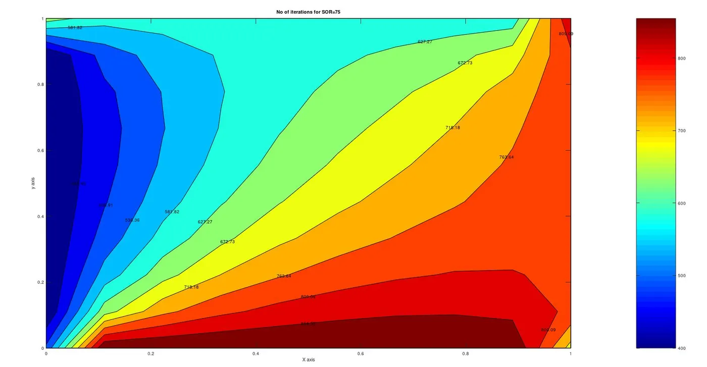
Code for Successive Over Relaxation method(SOR Method)
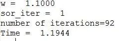
This method is an extrapolation of the Gauss Siedel method. Here `omega` is known as the extraplolation factor. When the value of `omega=1`, the following simplifies to the Gauss Siedel method.
The following equation is used to evaluate the solution:
`T_(i,j)=(1-omega)*Told_(i,j)+omega*(((T_(i-1,j)+Told_(i+1,j)) +(T_(i,j-1)+Told_(i,j+1)))/4);`
The above can be simplified as follows:
`T_(i,j)=(1-omega)*Told_(i,j) + omega*T_(GS)`
function T =sor_steady(error,tol,T,Told,i,j,nx,ny,x,y)
   w=1.1 % omega value
     sor_iter=1
     while(error>tol)
      for i=2:nx-1
        for j=2:ny-1
          T(i,j)=(1-w)*Told(i,j)+w*(((T(i-1,j)+Told(i+1,j)) +(T(i,j-1)+Told(i,j+1)))/4);
        end
       end
       error=max(max(abs(Told-T)));
       Told=T;
       sor_iter=sor_iter+1;


   end

   %Plot
   figure(3)
   contourf(x,y,T)
   [m n]=contourf(x,y,T);
   clabel(m,n);
   xlabel('X axis')
   ylabel('y axis')
   colormap(jet)
   colorbar

   title_text=sprintf('No of iterations for SOR=%d',sor_iter);
   title(title_text)

   pause(0.01)

 fprintf("number of iterations=%d n",sor_iter);
   endfunction
UNSTEADY/TRANSIENT STATE
The only difference between the steady state and unsteady state is that the variation of the heat is dependant on time.
The solution to this can be obtained in two ways.
- Explcit method (Does'nt require iterative solvers)
- Implicit method
EXPLICIT METHOD
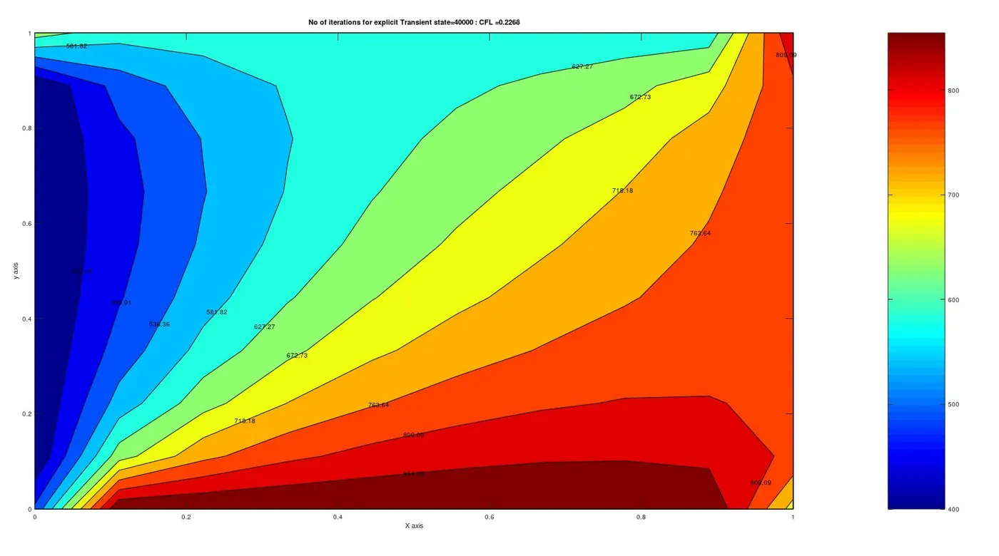
This method doesn't require the use of iterative solvers as solving this type of an equation yields the answer directly. In this method we evaluate the value of the temperature at the nth time step.
 %Explicit Method for transient state
 % domain is a unit square
 % nx=ny
 %boundary Conditions for steady and transient
 %T_left=400k
 %T_top=600k
 %T_right=800k
 %T_bottom=900k

 %*******************UNSteady State******************************

 % dT/dt=alpha*(d^2T/dx^2 +d^2T/dy^2)
 clear all
 close all
 clc
 % setting up length of domain and number of grid points
 L=1;
 nx=10;
 ny=nx;
 x=linspace(0,L,nx);
 dx=x(2)-x(1);
 y=linspace(0,L,ny);
 dy=y(2)-y(1);

 % time
 t=400;
 dt=1e-3;
 nt=t/dt

 % Setting the initial conditions
 T= ones(nx,ny)*298;

 T(:,1)=400; %left temp
 T(:,end)=800; %right temp
 T(end,:)=600; %top1 temp
 T(1,:)=900; %bottom temp

 % setting temperatures at either endswitch
 T(1,1)=(400+600)/2;
 T(nx,ny)=(800+900)/2;
 T(1,ny)=(600+800)/2;
 T(nx,1)=(400+900)/2;

 %Creating a copyfile
 Told=T;
 Tini=Told;
 error=9e9;
 tol=1e-4;
 alpha=1.7;
 [X,Y]=meshgrid(x,y);

 % in this case we consider the domain to be a square of dimension 1x1(m)
 % Also the number of grid points to be the same. Thus the value of the CFL NUmber would be the same

 % CFL number
 k1=(alpha*dt)/(dx)^2
 k2=(alpha*dt)/(dy)^2

 iter=1;
 tic;
 for m=  1:nt

   while (error>tol)
     for i= 2:nx-1
       for j= 2:ny-1
         T(i,j)=Told(i,j) + k1*(Told(i-1,j)+Told(i+1,j)-2*Told(i,j)) +k2*(Told(i,j+1)+Told(i,j-1)-2*Told(i,j));
       end
     end
     error=max(max(abs(Told-T)));
     Told=T;
     iter=iter+1;
   end
 end

  time=toc
  figure(1)
   contourf(x,y,T)
   [m n]=contourf(x,y,T);
   clabel(m,n);
   xlabel('X axis')
   ylabel('y axis')
   colormap(jet)
   colorbar

   title_text=sprintf('No of iterations for explicit=%d',iter);
   title(title_text)


   pause(0.01)

   fprintf("number of iterations=%d n",iter);
IMPLICIT METHOD
In this method the values of dependant vaariables are defiend by a set of equations thus we employ iterative techniques in order to obtain the solution.
Here we use three iterative techniques.
- Jocobi method
- Gauss Siedel method
- Successive over relaxation (SOR) method
MAIN PROGRAM
%Implicit Method for transient state
 % domain is a unit square
 % nx=ny
 %boundary Conditions for steady and transient
 %T_left=400k
 %T_top=600k
 %T_right=800k
 %T_bottom=900k

 %*******************UNSteady State******************************

 % dT/dt=alpha*(d^2T/dx^2 +d^2T/dy^2)
 clear all
 close all
 clc
 % setting up length of domain and number of grid points
 L=1;
 nx=10;
 ny=nx;
 x=linspace(0,L,nx);
 dx=x(2)-x(1);
 y=linspace(0,L,ny);
 dy=y(2)-y(1);

 % time
 t=400;
 dt=1e-5;
 nt=t/dt

 % Setting the initial conditions
 T= ones(nx,ny)*298;

 T(:,1)=400; %left temp
 T(:,end)=800; %right temp
 T(end,:)=600; %top1 temp
 T(1,:)=900; %bottom temp

 % setting temperatures at either endswitch
 T(1,1)=(400+600)/2;
 T(nx,ny)=(800+900)/2;
 T(1,ny)=(600+800)/2;
 T(nx,1)=(400+900)/2;

 %Creating a copyfile
 Told=T;
 Tprev=Told;
 error=9e9;
 tol=1e-4;
 alpha=1.7;
 [X,Y]=meshgrid(x,y);

 % in this case we consider the domain to be a square of dimension 1x1(m)
 % Also the number of grid points to be the same. Thus the value of the CFL NUmber would be the same

 % CFL number
 k1=(alpha*dt)/(dx)^2
 k2=(alpha*dt)/(dy)^2

 term1=1/(1+2*k1+2*k2);
 term2=k1*term1;
 term3=k2*term1;


 iter_sol=1:3;
 for iter_sol=1:3
   if iter_sol==1
     tic;
     T_jac = jocobi_implicit(error,tol,T,Told,i,j,nx,ny,x,y,term1,term2,term3,Tprev);
     Time=toc
    end

    if iter_sol==2
     tic;
     T_GS = GS_implicit(error,tol,T,Told,i,j,nx,ny,x,y,term1,term2,term3,Tprev);
     Time=toc
    end

    if iter_sol==3
     tic;
     T_sor = SOR_implicit(error,tol,T,Told,i,j,nx,ny,x,y,term1,term2,term3,Tprev);
     Time=toc
   end

  end
CODE FOR JOCOBI METHOD:
 % Function for jocobi method
 function T = jocobi_implicit(nt,error,tol,T,Told,nx,ny,x,y,term1,term2,term3,Tprev)
   j_iter=1;
   %Tprev=Told;

   for m=1:nt
     error=9e9;
     while(error>tol)
      for i=2:nx-1
        for j=2:ny-1
          H=Told(i-1,j)+Told(i+1,j);
          V=Told(i,j-1)+Told(i,j+1);
          T(i,j)=term1*Tprev(i,j)+term2*H+term3*V;
        end
       end
       error=max(max(abs(Told-T)));
       Told=T;
       j_iter=j_iter+1;

    end
  Tprev=T;
  end
   %Plot
   figure(1)
   contourf(x,y,T)
   [m n]=contourf(x,y,T);
   clabel(m,n);
   xlabel('X axis')
   ylabel('y axis')
   colormap(jet)
   colorbar

   title_text=sprintf('No of iterations for Jacobi_implicit=%d',j_iter);
   title(title_text)
   pause(0.03)

    fprintf("number of iterations=%d n",j_iter);

 endfunction
CODE FOR GAUSS SIEDEL METHOD:
 % Function for GS method
 function T = GS_implicit(nt,error,tol,T,Tprev,Told,nx,ny,x,y,term1,term2,term3)
   gs_iter=1
   for m=1:nt
     error=9e9;
     while(error>tol)
      for i=2:nx-1
        for j=2:ny-1
          H=T(i-1,j)+Told(i+1,j);
          V=T(i,j-1)+Told(i,j+1);
          T(i,j)=term1*Tprev(i,j)+term2*H+term3*V;
        end
       end
       error=max(max(abs(Told-T)));
       Told=T;
       gs_iter=gs_iter+1;

    end
    Tprev=T;
  end

   %Plot
   figure(3)
   contourf(x,y,T)
   [m n]=contourf(x,y,T);
   clabel(m,n);
   xlabel('X axis')
   ylabel('y axis')
   colormap(jet)
   colorbar

   title_text=sprintf('No of iterations for GS_implicit=%d',gs_iter);
   title(title_text)
   pause(0.03)

    fprintf("number of iterations=%d n",gs_iter);

 endfunction
CODE FOR SOR METHOD:
% Function for SOR method
 function T = SOR_implicit(error,tol,T,Told,i,j,nx,ny,x,y,term1,term2,term3,Tprev)
   sor_iter=1

   w=1.2

     while(error>tol)
      for i=2:nx-1
        for j=2:ny-1
          H=T(i-1,j)+Told(i+1,j);
          V=T(i,j-1)+Told(i,j+1);
          T_gs=term1*Tprev(i,j)+term2*H+term3*V;
          T(i,j)=(1-w)*Tprev(i,j)+w*T_gs;
        end
       end
       error=max(max(abs(Told-T)));
       Told=T;
       sor_iter=sor_iter+1;
       Tprev=T;
  end
   %Plot
   figure(2)
   contourf(x,y,T)
   [m n]=contourf(x,y,T);
   clabel(m,n);
   xlabel('X axis')
   ylabel('y axis')
   colormap(jet)
   colorbar

   title_text=sprintf('No of iterations for SOR_implicit=%d',sor_iter);
   title(title_text)
   pause(0.03)

    fprintf("number of iterations=%d n",sor_iter);

 endfunction
RESULTS:
The following are the findings.
STEADY STATE:
JACOBI METHOD:
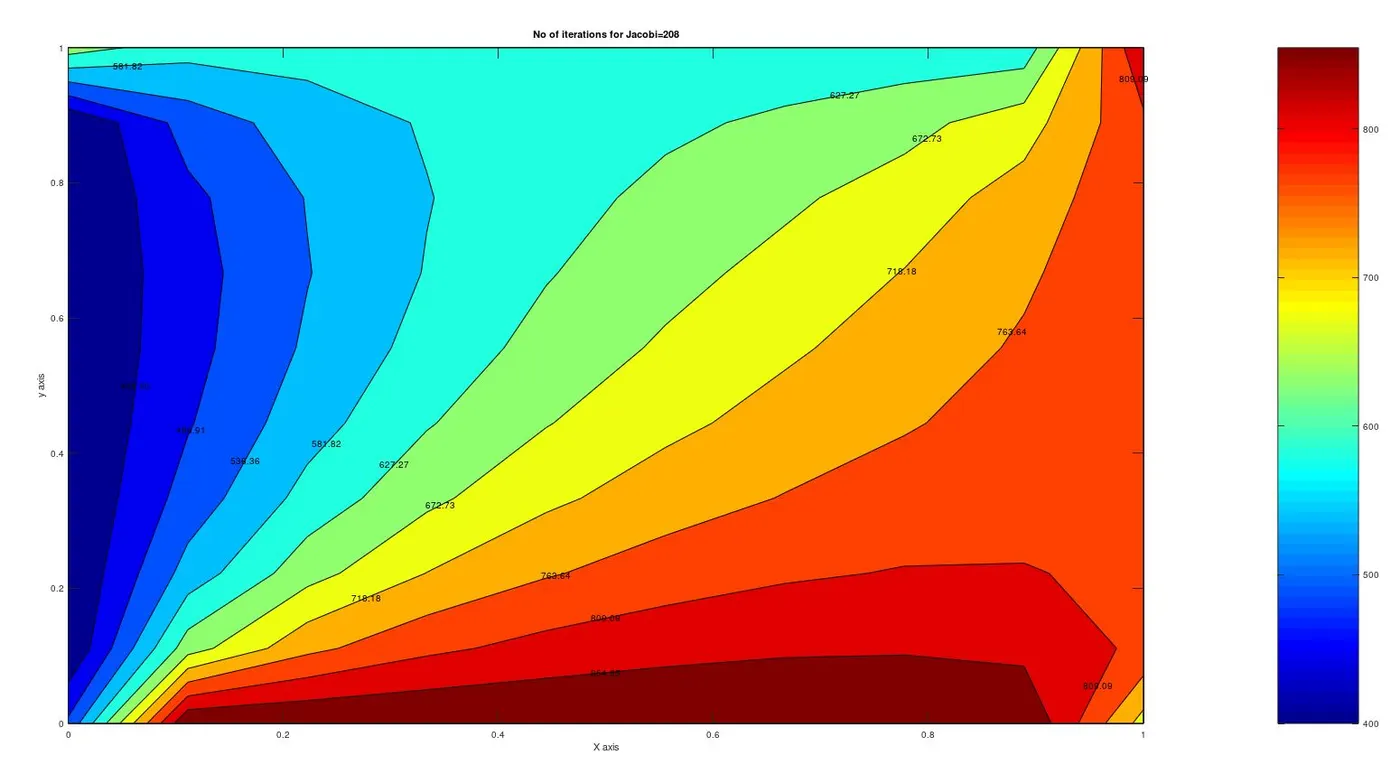
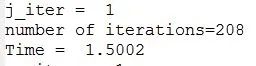
Time taken:
GAUSS SIEDEL METHOD:
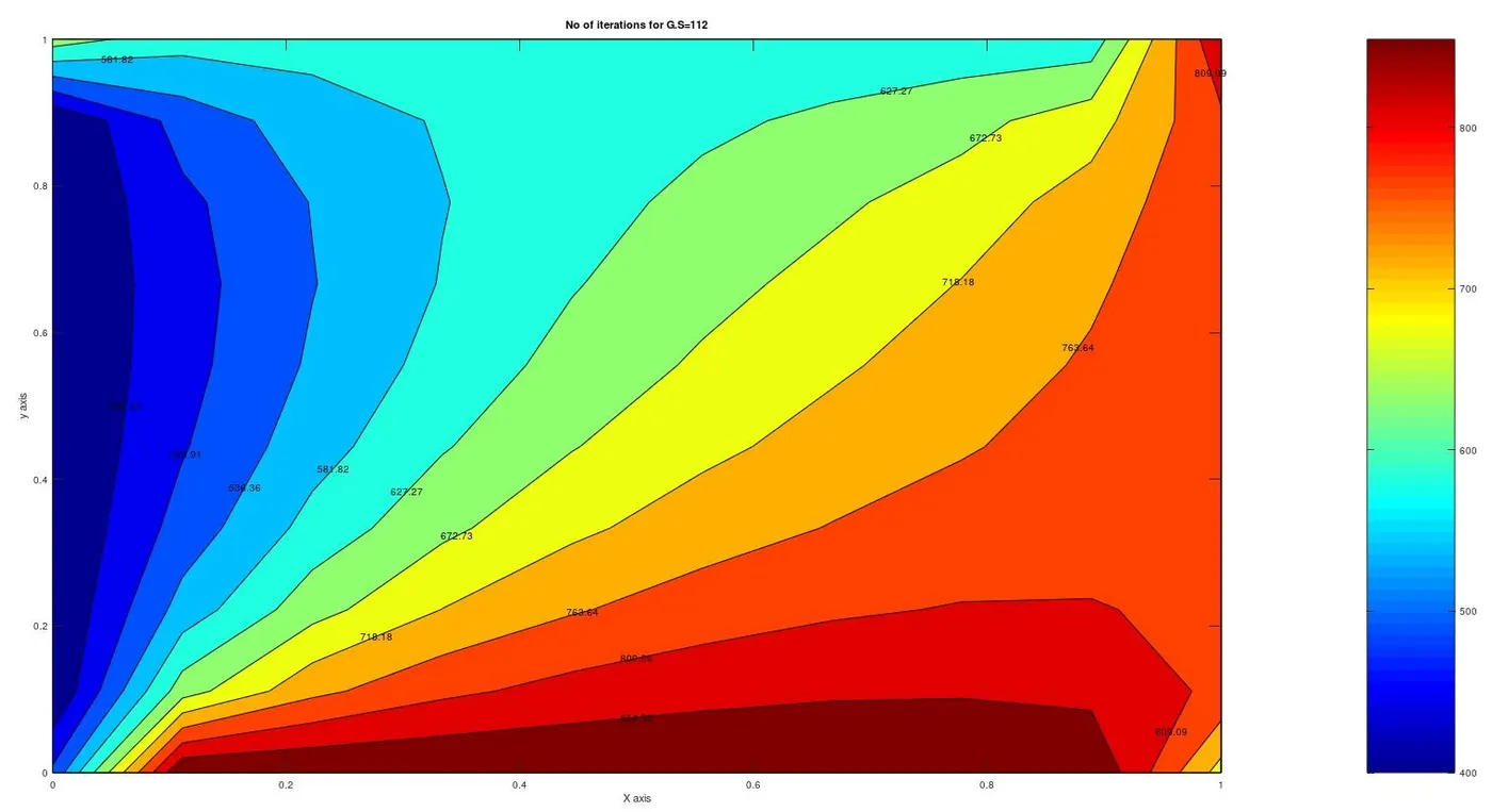
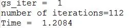
Time Taken:
SOR METHOD:
Time Taken:
TRANSIENT STATE
EXPLICIT METHOD:
Time Taken:
IMPLICIT METHOD
JACOBI METHOD:
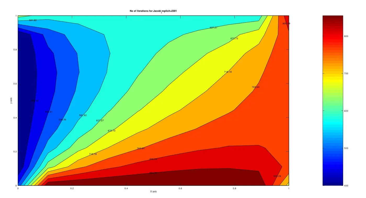
Time Taken:

GAUSS SIEDEL METHOD:
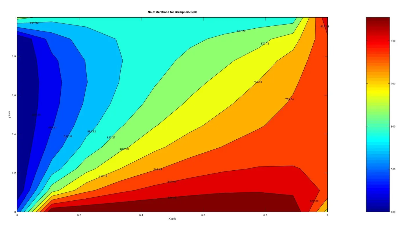
Time Taken:
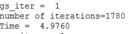
SOR METHOD:
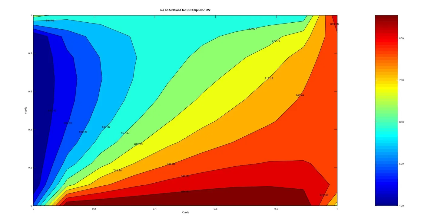
Time Taken:

INFERENCES:
From the above we can observe a certain trend. The trend is tabulated below.
|
Method of Iterative Solver used |
Steady State (iteration and time taken) |
Transient State Implicit(iteration and time taken) |
Transient State Explicit(iteration and time taken) |
|
Jocobi Method |
208 iterations and 1.5002 sec |
2301 iterations and 33.224 sec |
363 iterations and 1.3876 sec Iterative solvers were not used to evaluate the solution explicitly. |
|
Gauss Siedel Method |
112 iterations and 1.2084 sec |
1780 iterations and 4.9760 sec |
|
|
Successive Over Relaxation method(SOR) |
92 iterations and 1.1944 sec |
1322 iterations and 4.4514 sec |
From the above we can infer that SOR method is the most efficient method to evaluate the solution for the 2D conduction equaition because the solution converges in less number of iterations. Also it was found that if the value of `omega`lies between 0 and 2 the solution converges. However we require the solution to converge earliest. Thus the value of `omega` is set such that the same occurs. In this case we set `omega=1.1` in the case of steady state and `omega=1.2` in the case of transient state implicit method.
Thus we can infer that the efficiency of the iterative solvers is:
SOR>GS>Jocobi (in terms of efficiency).
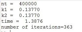
However, it can also be infered that the solution is reached sooner with less number of iteration in the explicit scheme. In the case of implicit versus explicit, the explicit converges sooner to the solution. Thus it seems to be efficient.