Week 9 - FVM Literature Review

Finite Volume Method:

The Finite volume method was introduced into the field of computational fluid dynamics at the beginning of the seventies(McDonald 1971, Mac Cormack and Paullay 1972). From the physical point of view, the FVM is based on balancing fluxes through control volumes.

In this scheme, the integral formulation of conservation laws are discretized directly in space. From the numerical analysis point of view, FVM is a generalization of the Finite difference method in geometrical and topological.

The finite volume method is a numerical technique used to solve partial differential equations that describe the physical phenomenon such as fluid flow, and heat transfer in a discretized domain. These techniques are widely used in computational fluid dynamics, computational heat transfer, and some related physical fields.

FVM has it's advantages and disadvantages. The advantages are FVM enforces the conservation of quantities at a discretized level. Fluxes between adjacent control volumes are directly balanced. Also, finite volume schemes take full advantage of arbitrary meshes to approximate complex geometries.

Differences between FVM and FDM:

Finite Volume Method	Finite difference Method
1. Discretization of the domain is based on the differential form of the PDE’s that are being solved	1. Discretization of the domain is based on the integral form of the PDE’s that are being solved
2. The finite-volume method is based on the fact that many physical laws are conservation laws—what goes into one cell on one side needs to leave the same cell on another side	2. In the equation all the derivatives are replaced with approximations based on Taylor series expansion.
3.The governing equations are solved for finite volume in which the discretized domain is represented in finite volumes.	3. The computational domain is mainly divided into grids, and governing equations are solved at nodes.
4. Does not require grid points	4. Requires grid points
5. Method is well versed in complex geometries.	5. This method is not appropriate for irregular geometries.
6. high resolution can be obtained	6. Resolution is based on the grid smoothness.

Finite Volume Method (FVM) with 1-D steady state heat conduction equation

ⅆ/ⅆx (k dT/dx)+s=0 1

Where k is thermal conductivity, T is temperature, and S is the rate of heat generation per unit volume.

To derive the discretization equation, let’s plot the grid points

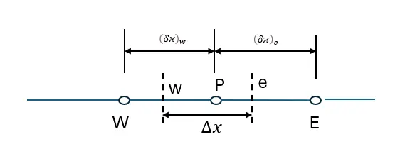
In this P is the particle (grid point) of interest and E and W are east and west side particles.

If we integrate Equation 1 within the control volume, we will get

(k ⅆT/ⅆϰ)_e-(k ⅆT/ⅆϰ)_w+∫_w^ⅇ▒sⅆx=0 2

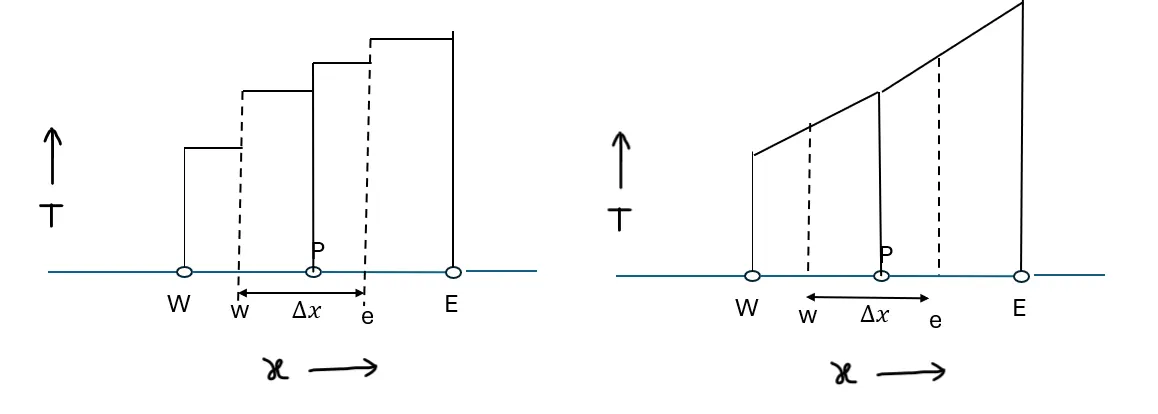
In the above picture, we can see the assumed step and piece-wise profiles for the interpolation. In these two profiles if we use stepwise interpolation the slope dt/dx is not defined at the control volume faces w and e. if we consider the piece wise interpolation it does not have this difficulty.

The discretized equation with piece-wise linear profile is as follows

(k_e (T_E-T_p ))/(δϰ)_e -(k_w (T_p-Tw))/(δx)w+s ̅Δx=0 3

Where s ̅ is the average value of s over the control volume. Now this equation can be represented as

a_p T_P=a_E T_E+a_w T_w+b

where

a_E=k_e/(δϰ)_e

a_w=k_w/(δϰ)_w

a_p= a_E+a_w

b=s ̅Δx

Guiding Principles:

There are different discretization formulations that we can choose from, we need to make sure as the grid points increase the solution does not change. Also, as coarser the grid gets the solution also should be physically realistic and overall balanced. The variations of physically realistic behavior is plotted below.

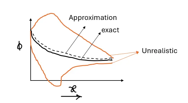
The formulation has four basic rules.

1. Consistency through control-volume faces: Two adjacent control volumes with a common face, the flux across it must be represented by the same expression in the discretization equations for the two control volumes.

2.Positive co-efficients: Most of these situations of interest will be in such a way where the value of dependent variable at a grid point is influenced by the values at neighboring grid points only through the process of convection and diffusion.

All coefficients always must be positive.

3. Negative slope linearization of source term: when the source term is linearized as

s ̅=s_c+ s_p T_P

This co-efficient s_palways be less than or equal to zero.

4. Sum of neighboring coefficients

We require

a_p=∑a_nb

For situations where the differential equation continues to remain satisfied after a constant is added to the dependent variable.

In this process, the next step will be the solution of the equations. The resulting system of linear equations is then solved to get the distribution of the required property at different nodal points. equations can be solved using any reasonable matrix-solving technique like AX = B.

Need for Interpolation schemes:

Evaluation of finite volume and surface integrals are required in FVM. The approximation of surface and volume integrals requires values of variables at locations other than the computational nodes of the control volume. For this, we need to come up with some mathematical or numerical schemes. That is the reason we need interpolation schemes.

Interpolation Schemes:

There are different interpolation schemes for different physical problems. Some of them are listed here

1. Upwind Interpolation

2. Linear Interpolation

3. Quadratic upwind Interpolation

Upwind Interpolation:

The upward interpolation scheme is essentially used for convection-dominated problems, and in these problems, The direction of the velocity at a given point determines the variable values used in the interpolation process.

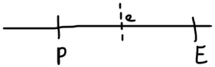
If we want to find the approximated value of a variable f at the east face of the control volume the formulation is as follows

f = f_p ⅈf(v⋅n)e>0

f_E ⅈf(v⋅n)e<0

The approximation values from this scheme are equivalent to backward or forward difference approximation depending upon the direction of the flow.

x---->

if the flow is in the negative direction of x, from the above formulation (v⋅n)e<0 means the interpolation is as follows

f_(i+1/2)≈f_i

f_(i-1/2)≈f_(i-1)

Approximation value = (f_i-f_(i-1))/Δx⋅v

which is a backward difference scheme. The vice versa for this formulation will be a forward difference scheme.

The advantage of this scheme is that only approximation satisfies boundedness numerically. The disadvantage is numerically diffusive and only first order accuracy.

Linear Interpolation:

The scheme is also known as the central difference scheme. Linear interpolation in the context of the finite volume method (FVM) is a technique used to approximate the values of a quantity at points within a control volume or on the faces of the control volume.

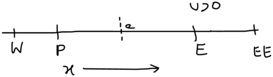
Now to approximate the value of the variable at control volume face by linear interpolation using the adjacent nodes is as follows.

x---->

Using the above notation from the picture

f_c=f_E ((ϰ_e-ϰ_p)/(x_E-ϰ_p ))+f_P ((ϰ_E-ϰ_e)/(x_E-ϰ_p ))

Important characteristics of the linear Interpolation scheme are

• Second-order accuracy
• Simplest and most widely used
• It might produce oscillations in the case of a coarse grid.

QUICK Interpolation:

This Interpolation was derived by Leonard in 1979, also named QUICK by him which is mainly applied to convective-dominated problems. This is a third-order accuracy model for both uniform and non-uniform grids. Being the 3rd-order accuracy model, it is widely applied to advection-dominated problems.

Now let’s look at the formulation for the QUICK scheme, approximation of the value of the variable at the control volume face by quadratic interpolation of the values using the three computational grid points is as follows

f=f_P+ϰ_f (f_E-f_p )+x_g (f_w-f_p )

x_f=((ϰ_e-ϰ_p)/(x_E-ϰ_p ))((ϰ_e-ϰ_w)/(x_E-ϰ_w ))

x_g=((ϰ_e-ϰ_p)/(x_W-ϰ_p ))((ϰ_e-ϰ_E)/(x_W-ϰ_E ))

The advantage of QUICk compared to upwind and linear schemes is more accurate and more damped.

There are some other schemes Hybrid Interpolation(which is a combination of linear and upwind schemes), and Total Variation diminishing (TVD)scheme.

In the TVD scheme, we will come across a function called the flux limiter function. Which is denoted by ψ.

Flux Limiter:

In the finite volume method (FVM), a flux limiter is a technique used to stabilize the solution, particularly in scenarios where sharp gradients or discontinuities exist in the solution. Flux limiters are employed to prevent oscillations or numerical instabilities that may arise when solving hyperbolic partial differential equations (PDEs) using finite volume discretization.

Here's why flux limiters are necessary

Sharp Gradients and Discontinuities: In many physical phenomena, sharp gradients or discontinuities may occur in the solution. These could be due to shock waves, material interfaces, or other abrupt changes in the solution field.

Numerical Instabilities: When solving hyperbolic PDEs with finite volume methods, numerical schemes may encounter difficulties in accurately representing these sharp gradients or discontinuities. This can lead to oscillations, smearing of features, or even outright instability of the numerical solution.

In FVM, fluxes represent the flow of quantities (such as mass, momentum, or energy) across control volume interfaces. Accurate computation of fluxes is crucial for capturing the correct physics of the problem. Flux limiters are introduced to constrain the magnitude of the computed fluxes, particularly in regions where sharp gradients or discontinuities are present. By limiting the fluxes, these methods effectively dampen excessive oscillations and prevent numerical instability.

Just for the clarity of equations I did upload the Word document.

References:

1. Numerical heat transfer and fluid flow by Suhas v.Patankar

2. Computational fluid dynamics by Chung, T.J 2nd edition