Project 2 - Rankine cycle Simulator
Rankine Cycle:
Rankine cycle, which is the ideal cycle for vapor power plants. The ideal Rankine cycle does not involve any internal irreversibilities and consists of the following four processes:
1-2 Isentropic compression in a pump
2-3 Constant pressure heat addition in a boiler
3-4 Isentropic expansion in a turbine
4-1 Constant pressure heat rejection in a condenser
Assumptions for the problem:
1 Steady operating conditions exist.
2 Kinetic and potential energy changes are negligible.
The Rankine cycle consists of four distinct processes:
-
Isentropic Expansion: In this phase, steam is introduced into a turbine where it undergoes expansion. As a result, both pressure and temperature of the steam decrease. This expansion process drives the turbine, producing electricity.
-
Constant Pressure Heat Rejection: Wet steam, which has gone through the expansion phase, releases heat into a condenser. During this stage, the phase of the steam changes, and it transforms into saturated liquid.
-
Isentropic Compression: Water is pumped from a low-pressure region to a high-pressure region through an isentropic process. This pumping operation requires some input energy.
-
Constant Pressure Heat Addition: Water is supplied to a boiler, where it is heated until it reaches the phase of dry saturated vapor. This heating process takes place at a constant pressure, and heat is added to the water, making it dry saturated vapor.
Assumptions for the problem:
1 Steady operating conditions exist.
2 Kinetic and potential energy changes are negligible.
Output Parameters:
heat addition = h1−h4
heat rejection = h2−h3
work done by turbine(wt) = h1−h2
work taken by pump (wp) = h4−h3
thermal efficiency = (wt–wp)/heat addition
net work output= wt-wp
back work ratio(BWR) = wp/wt
Code for the Rankine cycle:
I did use copy and paste because insert code option is not available in the new interface.
clear
close all
clc
fprintf(" RANKINE CYCLE SIMULATOR \n")
fprintf('Process 1-2: Isentropic Expansion in Turbine \n')
fprintf('Process 2-3: Constant Presssure Heat Rejection in Condenser \n')
fprintf('Process 3-4: Isentropic Compression in Pump \n')
fprintf('Process 4-1: Constant Presssure Heat Addition in Boiler \n')
% input parameters
p1=input('Enter the pressure at the Turbine inlet (bar):');
t1=input('Enter the Turbine inlet temperature (in degrees celcius):');
p2=input('Enter the condenser inlet Pressure (bar):');
% variables for state1
h1 = XSteam('h_pT',p1,t1); % Enthalpy values at p1 & t1
s1 = XSteam('s_ph',p1,h1); % Entropy values at p1 & h1
%Printing the values at state 1
fprintf('\n\n Results')
fprintf('\n\n At state point 1')
fprintf('\n P1 is:�ar',p1)
fprintf('\n T1 is:�eg celcius',t1)
fprintf('\n H1 is:%f KJ/Kg',h1)
fprintf('\n S1 is:%f KJ/KgK',s1)
% Variables for state2
s2 = s1; % Entropy value at stage 2
t2 = XSteam('T_ps',p2,s2); % Temperature at p2 & s2
sf2 = XSteam('sL_p',p2); % Saturated liquid entropy at state2
sg2 = XSteam('sV_p',p2); % Saturated vapour entropy at state2
hf2 = XSteam('hL_p',p2); % Saturated liquid enthalpy at state2
hg2 = XSteam('hV_p',p2); % Saturated vapour enthalpy at state2
x = ((s2 - sf2)/(sg2 - sf2)); % vapour fraction
h2 = hf2 + (x*(hg2 - hf2)); % enthalpy at state2
v2 = XSteam('v_ph',p2,h2); % volume at state2
%Printing the values at stage 2
fprintf('\n\n At state point 2')
fprintf('\n P2 is:�ar',p2)
fprintf('\n T2 is:�eg celcius',t2)
fprintf('\n H2 is:%f KJ/Kg',h2)
fprintf('\n S2 is:%f KJ/KgK',s2)
% variables for state3
t3 = t2; % Temperature at state3
p3 = p2; % Pressure at state 3
s3 = XSteam('sL_p',p3); % Entropy at pressure p3
h3 = XSteam('hL_T',t3); % Enthalpy at temperature t3
v3 = XSteam('v_ph',p3,h3); % volume at state3
%Printing the values at state 3
fprintf('\n\n At state point 3')
fprintf('\n P3 is:�ar',p3)
fprintf('\n T3 is:%f deg celcius',t3)
fprintf('\n H3 is:%f KJ/Kg',h3)
fprintf('\n S3 is:%f KJ/KgK',s3)
% variables for state4
s4 = s3; % Entropy at state4
v4 = v3; % volume at state4
p4 = p1; % pressure at state4
h4 = XSteam('h_ps',p4,s4); % enthalpy at state4
t4 = XSteam('T_hs',h4,s4); %Temperature at state4
% Printing the values at state4
fprintf('\n\n At state point 4')
fprintf('\n P4 is:�ar',p4)
fprintf('\n T4 is:�eg celcius',t4)
fprintf('\n H4 is:%f KJ/Kg',h4)
fprintf('\n S4 is:%f KJ/KgK',s4)
% variables for stage5
p5 = p4; % Pressure at state 5
t5 = XSteam('Tsat_p',p5); % saturation temperature at state 5
h5 = XSteam('hL_T',t5); % Enthalpy at state 5
s5 = XSteam('sL_p',p5); % Entropy at state 5
% Printing the values at state5
fprintf('\n\n At state point 5')
fprintf('\n P5 is:�ar',p5)
fprintf('\n T5 is:�g celcius',t5)
fprintf('\n H5 is:%f KJ/Kg',h5)
fprintf('\n S5 is:%f KJ/KgK',s5)
% variables for stage6
t6 = t5; % Temperature at state 6
p6 = XSteam('psat_T',t5); %Pressure at state 6
s6 = XSteam('sV_T',t6); %Entropy at state 6
h6 = XSteam('hV_T',t6); % Enthalpy at state 6
% Printing the values at state6
fprintf('\n\n At state point 6')
fprintf('\n P6 is:�ar',p6)
fprintf('\n T6 is:�eg celcius',t6)
fprintf('\n H6 is:%f KJ/Kg',h6)
fprintf('\n S6 is:%f KJ/KgK',s6)
% loop to find variables on saturation lines
t = linspace(0,400,1000);
%Entropy and Enthalpy calculations for liquid and vapour states
for i=1:length(t)
s_line1(i)=XSteam('sL_T',t(i));
end
for j=1:length(t)
s_line2(j)=XSteam('sV_T',t(j));
end
for i=1:length(t)
h_line1(i)=XSteam('hL_T',t(i));
end
for j=1:length(t)
h_line2(j)=XSteam('hV_T',t(j));
end
% net work output calculation
w_turbine = h1 - h2; % work done by turbine
w_pump = h4 - h3; % work taken by pump
work = w_turbine - w_pump; % net work output
q_in = h1 - h4; % heat addition
q_out = h2 -h3; % heat rejection
% thermal efficiency
n = work/q_in;
�ck work ratio
BWR = w_pump/w_turbine;
%Printing the values for output values
fprintf('\n\n Output values')
fprintf('\n\n w_turbine is:%f ',w_turbine)
fprintf('\n w_pump is:%f ',w_pump)
fprintf('\n Net work output is:%f ',work)
fprintf('\n Heat added to the system is :%f ',q_in)
fprintf('\n Heat removed from the system is :%f ',q_out)
fprintf('\n Therml efficiency of the system is :%f ',n)
fprintf('\n Back work ratio of the system is:%f ',BWR)
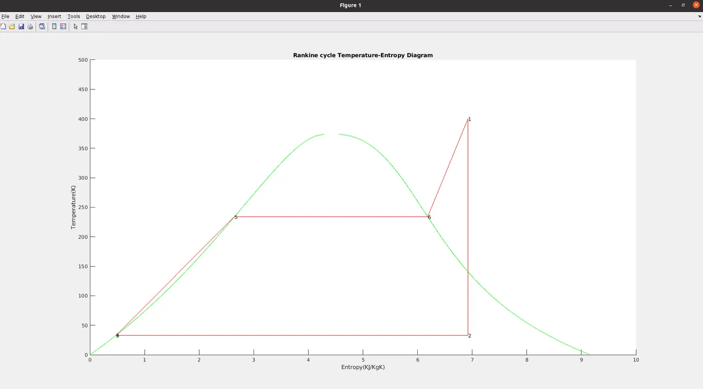
%plotting Temperature-Entropy graph
figure(1)
hold on
%fine colors for lines
lineColor1 = 'green'; % For the first line
lineColor2 = 'red'; % For the second line
plot([s_line1 s_line2], [t t], 'Color', lineColor1)
plot([s1 s2 s3 s4 s5 s6 s1], [t1 t2 t3 t4 t5 t6 t1], 'Color', lineColor2)
% plot([s_line1 s_line2],[t t])
% plot([s1 s2 s3 s4 s5 s6 s1],[t1 t2 t3 t4 t5 t6 t1])
text(s1,t1,'1')
text(s2,t2,'2')
text(s3,t3,'3')
text(s4,t4,'4')
text(s5,t5,'5')
text(s6,t6,'6')
title("Rankine cycle Temperature-Entropy Diagram")
xlabel('Entropy(KJ/KgK)')
ylabel('Temperature(K)')
axis([0,10,0,500])
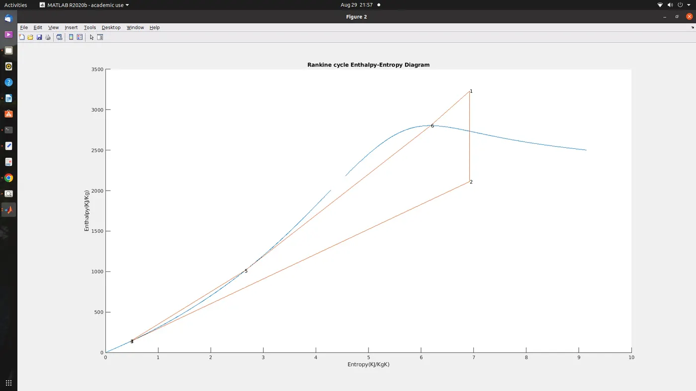
%plotting enthalpy-entropy graph
figure(2)
hold on
% plot([s_line1 s_line2], [t t], 'Color', lineColor3)
% plot([s1 s2 s3 s4 s5 s6 s1], [t1 t2 t3 t4 t5 t6 t1], 'Color', lineColor4)
plot([s_line1 s_line2],[h_line1 h_line2])
plot([s1 s2 s3 s4 s5 s6 s1],[h1 h2 h3 h4 h5 h6 h1])
text(s1,h1,'1')
text(s2,h2,'2')
text(s3,h3,'3')
text(s4,h4,'4')
text(s5,h5,'5')
text(s6,h6,'6')
title("Rankine cycle Enthalpy-Entropy Diagram")
xlabel('Entropy(KJ/KgK)')
ylabel('Enthalpy(KJ/Kg)')
axis([0,10,0,3500])
Errors in the Program:
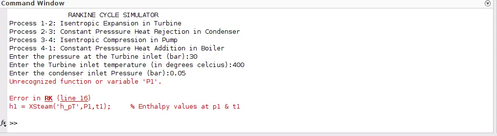
Error1:Urecognized function or variable P1(This type of error occured three times more but did not included due same error and solution)
Solution: changed P1 to p1
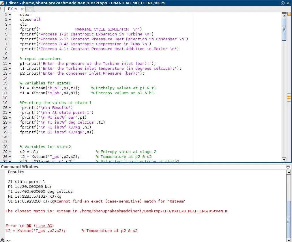
Error2 : cannot find an exaxct (case-sensitive) match for 'Xsteam'(This error also occured two to three times but only attached once)
Solution: chanaged Xsteam to XSteam
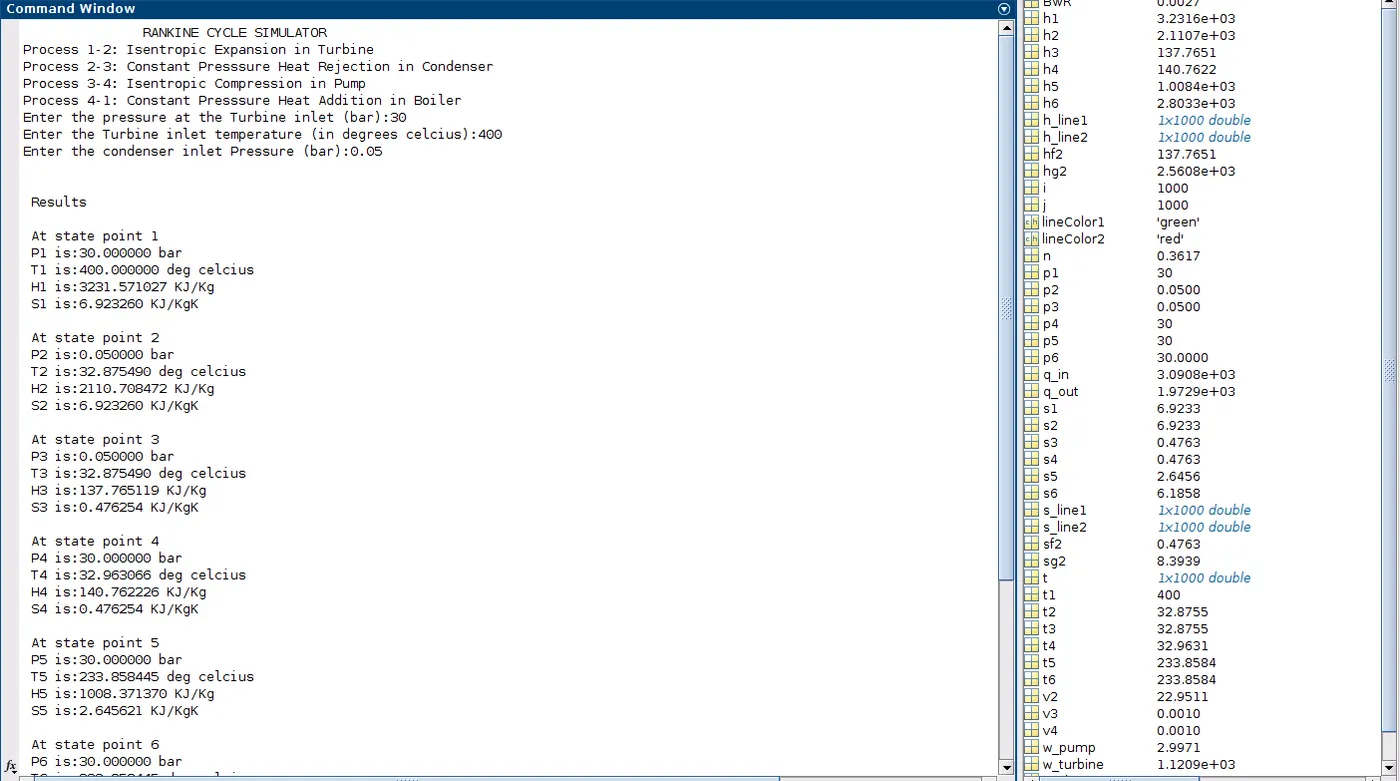
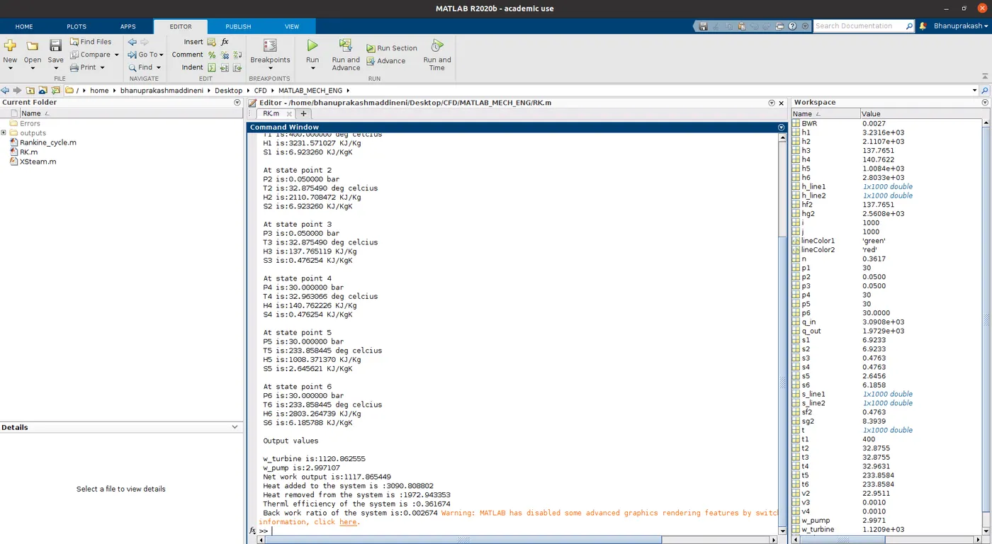
Output:
In the command window
T-S Graph
h-s Graph:
Conclusion:
based on the rankine cycle if we give the initial pressure p1 and T1 and P2 the code will be able to calculate all the state values at each state and the output values.After this the graphs are plotted between T-S and h-s.
The Interface of the browser skill lync has been changed.I did follow the instructions to make the report as accurate as possible.please let me know if something is missing on your end. I did attached the errors, output form command window and graphs of T-s and h-s.