Week 3.5 - Deriving 4th order approximation of a 2nd order derivative using Taylor Table method

All of the derivations are done by hand and uploaded as a PDF to save time in typing the equations.

Here is the Matlab code used to solve for the values from the 3 derivations of the Taylor table.

clear 
close all
clc

A1 =[1 1 1 1 1; -2 -1 0 1 2;2 0.5 0 0.5 2;-4/3 -1/6 0 1/6 4/3;2/3 1/24 0 1/24 2/3];

B1 = [0 0 1 0 0]';

X = linsolve(A1,B1);
%%
clear 
close all
clc

A1 =[1 1 1 1 1 1; 0 1 2 3 4 5; 0 1/2 2 4.5 8 12.5;
    0 1/6 4/3 9/2 32/3 125/6;
    0 1/24 2/3 81/24 32/3 625/24;
    0 1/120 4/15 81/40 128/15 625/24];
B1 = [0 0 1 0 0 0]';

X1 = linsolve(A1,B1);

%%
clear 
close all
clc

A2 =[1 1 1 1 1 1;-5 -4 -3 -2 -1 0;12.5 8 4.5 2 1/2 0;
     -125/6 -32/3 -9/2 -4/3 -1/6 0;
     625/24 32/3 81/24 2/3 1/24 0;
     -625/24 -128/15 -81/40 -4/15 -1/120 0];
B2 = [0 0 1 0 0 0]';

X2 = linsolve(A2,B2);

Here I separated each section and ran the section for the results. or we can delete the sections and remove clear close all and clc from the bottom two sections and we can run the entire code one time to get the results.

The next objective is to write the MATLAB code evaluate exp(x)*cos(x) for all of these 3 numerical approximations derived

Here is the code for the analytical and 3 numerical approximations error comparison

clear
close all
clc

% Function that need to be analyzeed
%f(x)=exp(x)*cos(x)
% analytical derivative=-2*sin(x)*exp(x)

% input values
x = pi/3;

%dx values
dx = linspace(pi/40,pi/4000,100);


% for loop for calculating the numerical approximations
for i =1:length(dx)
    
   [central_error(i),right_error(i),left_error(i)] = taylor_table_values(x,dx(i));

end

%Slope of the central order error line
slope_1=diff(central_error)/diff(dx);

%Slope of the right skewed
slope_2=diff(right_error)/diff(dx);

%Slope of the left skewed
slope_3=diff(left_error)/diff(dx);


%loglog plot of errors vs dx
figure(1)
loglog(dx,central_error)
hold on
loglog(dx,right_error)
loglog(dx,left_error)
hold off
xlabel('dx')
ylabel('error')
title('error comparison for different approximation schemes')
legend('central error','right skewed error','left skewed error')

function [central_error,right_error,left_error] =taylor_table_values(x,dx)
% values for co-efficients central difference
a =-0.0833;
b = 1.3333;
c =-2.5000;
d =1.3333;
e = -0.0833;

% values for co-efficients right skewed
  a1 =  3.75;
  b1 =  -12.8333;
  c1 =  17.8333;
  d1 = -13.00;
  e1 =  5.0833;
  f1 =  -0.833;

% values for co-efficients left skewed
a2 = -0.8333;
 b2 = 5.0833;
 c2 = -13.00;
 d2 = 17.833;
 e2 = -12.8333;
 f2 = 3.750;

%Numericl approximation using fourth order central difference approximation
derivative = (a*exp(x-(2*dx))*cos(x-(2*dx))+b*exp(x-dx)*cos(x-dx)+c*exp(x)*cos(x)+d*exp(x+dx)*cos(x+dx)+e*exp(x+(2*dx))*cos(x+(2*dx)))/(dx^2);

%Numericl approximation using fourth order central difference approximation
derivative_1 = ((a1*(exp(x)*cos(x)))+(b1*(exp(x+dx)*cos(x+dx)))+(c1*(exp(x+(2*dx))*cos(x+(2*dx))))+(d1*(exp(x+(3*dx))*cos(x+(3*dx))))+(e1*(exp(x+(4*dx))*cos(x+(4*dx))))+(f1*(exp(x+(5*dx))*cos(x+(5*dx)))))/(dx)^2;

%Numericl approximation using fourth order central difference approximation
derivative_2 = ((a2*(exp(x-(5*dx))*cos(x-(5*dx))))+(b2*(exp(x-(4*dx))*cos(x-(4*dx))))+(c2*(exp(x-(3*dx))*cos(x-(3*dx))))+(d2*(exp(x-2*dx)*cos(x-(2*dx))))+(e2*(exp(x-(1*dx))*cos(x-(1*dx))))+(f2*(exp(x)*cos(x))))/(dx)^2 ;

analytical = -2*sin(x)*exp(x);

%error in central difference scheme
central_error = abs(analytical-derivative);

%error in right skewed  scheme
right_error = abs(analytical-derivative_1);

%error in left  skewed  scheme
left_error = abs(analytical-derivative_2);
end

The code results are attached as a pdf. Here is the Graph for the errors between fourth-order central approximation, right-skewed approximation, and left-skewed approximation.

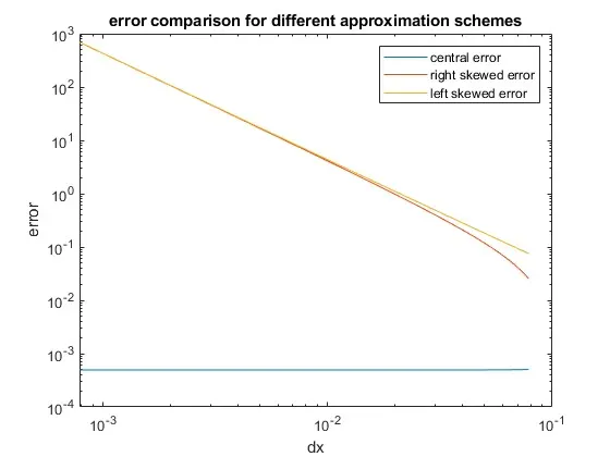
From the graphs, we can see that the central difference scheme has the lowest error in all of the approximations.

Describe why a skewed scheme is useful. What can a skewed scheme do that a CD scheme cannot?

Ans: Skewed schemes are useful in the case the nodes end at the end of the grids there won't be any nodes to the right or the left.Where the boundaries are present. So in the case of these boundaries, the skewed systems will play a key role in evaluating the property. This is what a skewed system can do that CDS cannot. But if we have internal nodal points available CDS works very well.