Week 9 - FVM Literature Review

AIM: Finite Volume Method

1. What is the Finite Volume Method(FVM),
2. Major differences between FDM & FVM
3. Need for interpolation schemes and flux limiters in FVM.

INTRODUCTION:

The Finite Volume (or control volume) Method or FVM is a numerical technique that transforms the partial differential equations representing conservation laws over differential volumes into discrete algebraic equations over finite volumes (or elements or cells). The first step in the solution process is the discretization of the geometric domain, which, in the FVM, is discretized into non-overlapping elements or finite volumes. The partial differential equations are then discretized/transformed into algebraic equations by integrating them over each discrete element. The system of algebraic equations is then solved to compute the values of the dependent variable for each of the elements.

In FVM, some of the terms in the conservation equation are turned into face fluxes and evaluated at the finite volume faces. As the flux entering a given volume is identical to that leaving the adjacent volume, the FVM is strictly conservative. This inherent conservation property makes it the preferred method in CFD. Another important attribute of the FVM is that it can be formulated in the physical space on unstructured polygonal meshes. It is also quite easy to implement a variety of boundary conditions in a non-invasive manner, since the unknown variables are evaluated at the centroids of the volume elements, not at their boundary faces.

These characteristics have made FVM quite suitable for the numerical simulation of a variety of applications involving fluid flow and heat and mass transfer, and developments in the method have been closely entwined with advances in CFD. From a limited potential at inception confined to solving simple physics and geometry over structured grids, the FVM is now capable of dealing with all kinds of complex physics and applications.

The finite volume method is developed for this study considering the one-dimensional steady-state heat conduction equation

`\frac{\partial }{\partial x} ( \alpha \frac{\partial T}{\partial x} ) + S = 0`

`rarr1`

where `k` is the thermal conductivity, the dependent variable is temperature `T`, and `S` is the source term.

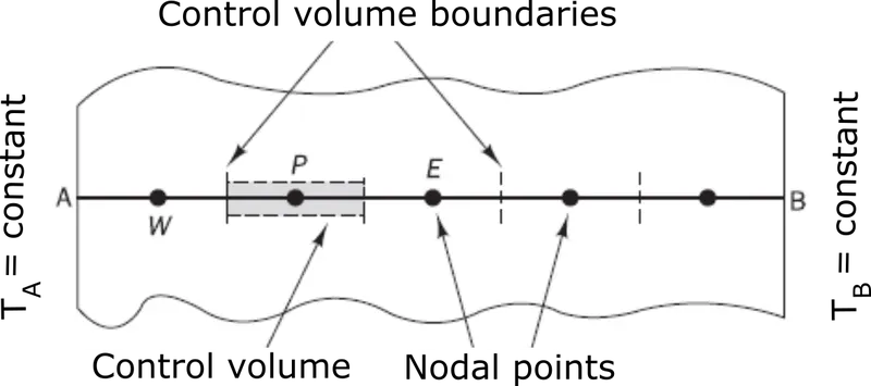Figure 1

Step 1: Grid generation

The domain is split into discrete control volumes as the first stage in the finite volume approach. In the region between points A and B, several nodal points are positioned. Control volume boundaries (or faces) are positioned halfway between neighboring nodes. Thus, a control volume or cell surrounds each node. It is standard procedure to arrange control volumes close to the domain's edge so that their bounds align with the physical ones. Now is the time to create a notational framework that can be applied to future developments. Figure 2 depicts the typical CFD technique convention.

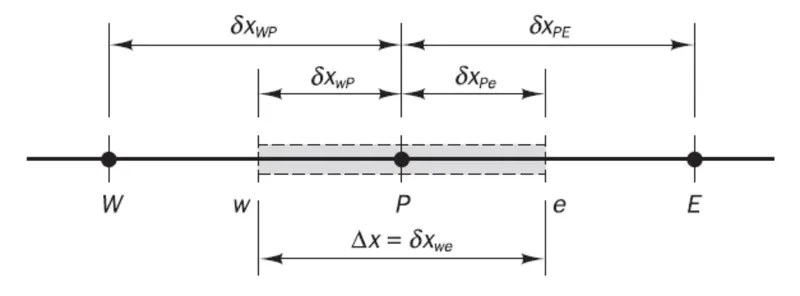Figure 2

In a one-dimensional geometry, a general nodal point is denoted by P, while its neighbors, the nodes to the west and east, are denoted by W and E, respectively. The east side control volume face is denoted by `e`, and the west side control volume face is denoted by `w`. `deltax_(WP)` and `deltax_(Pe)`, respectively, stand for the distances between the nodes W and P and between the nodes P and E. Similar distances between face `w` and point P and between P and face `e` are indicated, respectively, by the symbols `deltax_(WP)` and `deltax_(PE)`. The width of the control volume is depicted as `Deltax = deltax_(we)` in Figure 2.

Step 2: Discretization

The integration of the governing equation (or equations) over a control volume to produce a discretized equation at its nodal point P is the crucial step in the finite volume approach. This results for the control volume described above.

	`\int \frac{\partial }{\partial x}( \alpha \frac{\partial T}{\partial x} ).dV+\int S.DeltaV=0`
`rArr`	`\int \frac{\partial }{\partial x}( \alpha \frac{\partial T}{\partial x} ).Adx+\int S.DeltaV=0`

Here `A` is the cross-sectional area of the control volume face, `dV` is the volume and `barS` is the average value of source `S` over the control volume.

	`[ \alpha A\frac{\partial T}{\partial x} ]_{e}^{w}+barS.DeltaV=0`
`rArr`	`[ \alpha_w A\frac{\partial T}{\partial x_w}]-[ \alpha_e A\frac{\partial T}{\partial x_e}] +barS.DeltaV=0`	`rarr 2`

The discretized equation's clear physical explanation makes the finite volume technique particularly appealing. Equation `2` states that a balance equation over the control volume is formed by the heat flux leaving the east face minus the heat flux entering the west face.

The gradient `(dT)/dx` at the east (`e`) and west (`w`) as well as the thermal conductivity `alpha` is needed to develop practical forms for the discretized equations. An approximation of the distribution of characteristics among the nodal points is used to calculate the gradients (and subsequently the fluxes) at the control volume faces. The most obvious and straightforward method of determining interface values and gradients appears to be linear approximations.

`alpha_w = (alpha_W+alpha_P)/2`	`rarr 3.a`
`alpha_e = (alpha_P+alpha_E)/2`	`rarr 3.b`

The flux terms are evaluated as-

`alpha_eA(dT)/(dx_e)=alpha_eA((T_E-T_P)/(delx_(PE)))`	`rarr 4.a`
`alpha_wA(dT)/(dx_w)=alpha_wA((T_P-T_w)/(delx_(WP)))`	`rarr 4.b`

The source term `S` would be a function of the dependent variable in practical situations. In this case, the finite volume method approximates the source by means of a linear form:

`barSDelta V = S_u +S_pT_p`

`rarr 5`

Substituting equations `3`, `4`, and `5` into equation `2` gives

`((alpha_e)/(deltax_(PE))A+(alpha_w)/(deltax_(WP))A-S_p)T_P=((alpha_w)/(deltax_(WP))A)+((alpha_e)/(deltax_(PE))A)T_E+S_u`

`rarr 6`

Equation `6` can be expressed by identifying the coefficients of `T_P`, `T_W`, and `T_E` as `a_P`,`a_W`, and `a_E` respectively as

`a_PT_P=a_WT_W+a_ET_E+S_u`

`rarr 7`

Step3: Solution of equations

At each of the nodal points, discretized equations of form `7` must be put up in order to solve a problem. The general discretized equation `7` is changed to include boundary conditions for control volumes that are adjacent to the domain boundaries. The distribution of the temperature T at nodal sites is then determined by solving the ensuing system of linear algebraic equations. For this purpose, any acceptable matrix solution method may be used.

Now, let us discuss how the Finite Volume Method (FVM) is different from the Finite Difference Method (FDM).

Finite Volume Method (FVM)	Finite Difference Method (FDM)
Integral form of governing equations `\oint \oint \frac{\partial f}{\partial x}dxdy=\oint fdy=C*Area`	Differential from of governing equations `\frac{\partial f}{\partial x}=(f_(i+1)-f_i)/(Deltax)=C`
Domain is discretized into finite volumes.	Domain is discretized into finite discrete points.
Properties are calculated for every cell based.	Properties are calculated for every cell every node based.
The discretization technique uses fluxes through volumes, i.e. Gauss's divergence theorem.	The discretization technique is using Taylor series.
Defined on any irregular/unstructured grid.	Defined on a regular/structured grid.
Grid smoothness is not required since independent variables are integrated directly on the physical domain.	Depends on grid smoothness.
Highly refined mesh can be obtained at the corners.	Adaptive mesh refinement is not possible.

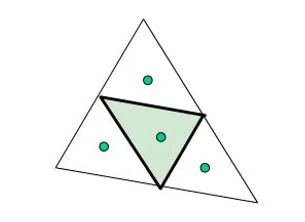
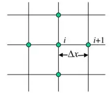
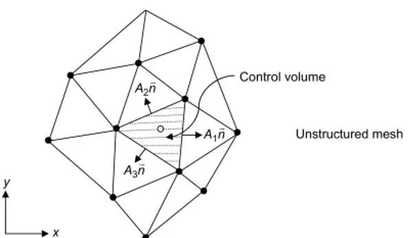
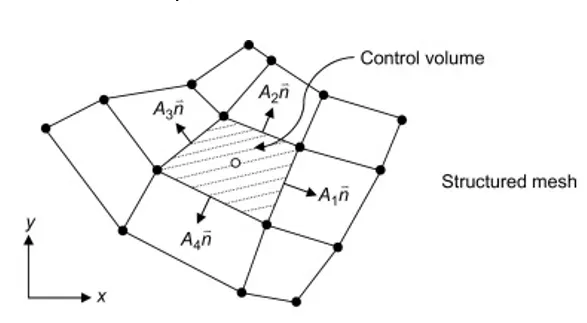
Interpolation schemes are used to transform cell-center quantities to face centers. The operation is used in many of the finite volume calculations, e.g. for the calculation of gradient, divergence, and Laplacian terms.

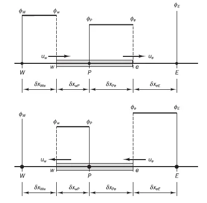
Upwind interpolation scheme - The upwind differencing or ‘donor cell’ differencing scheme takes into account the flow direction when determining the value at a cell face: the convected value of `phi` at a cell face is taken to be equal to the value at the upstream node. In Figure 3 (top) we show the nodal values used to calculate cell face values when the flow is in the positive direction (west to east) and in Figure 3 (bottom) those in the negative direction.

Figure 3

When the flow is in the positive direction, `u_w>0, u_e>0 (F_w>0,F_e>0), the upwind scheme sets

`phi_w=phi_W` and `phi_e=phi_P`

and the discredited equation becomes

`[(D_w+F_w)+D_e+(F_e-F_w)] phi_P=(D_w+F_w)phi_W+D_ephi_E`

When the flow is in the negative direction, `u_w<0, u_e<0 (F_w<0,F_e<0), the scheme takes

`phi_w=phi_P` and `phi_e=phi_E`

Now, the discretized equation is

`[D_w+(D_e-F_e)+(F_e-F_w)] phi_P=D_wphi_W+(D_e-F_e)phi_E`

Identifying the coefficients of `phi_W`and `phi_E` as `a_W` and `a_E`, the discretized equation can be written in the usual general form

`a_pphi_p=a_Wphi_W+a_Ephi_E`

Some of the other interpolation schemes used in CFD are:

• Linear interpolation scheme
• Hybrid differencing scheme
• Power-law scheme
• Quadratic upwind differencing scheme (QUICK scheme)
• Total variation diminishing or TVD

Flux Limiter: a switch

The main idea behind the construction of flux limiter schemes is to limit the spatial derivatives to realistic values - for scientific and engineering problems, this usually means physically realizable values. They are used in high-resolution schemes for solving problems described by PDEs and only come into operation when sharp wavefronts are present. For smoothly changing waves, the flux limiters do not operate, and the spatial derivatives can be represented by higher-order approximations without introducing nonreal oscillations.

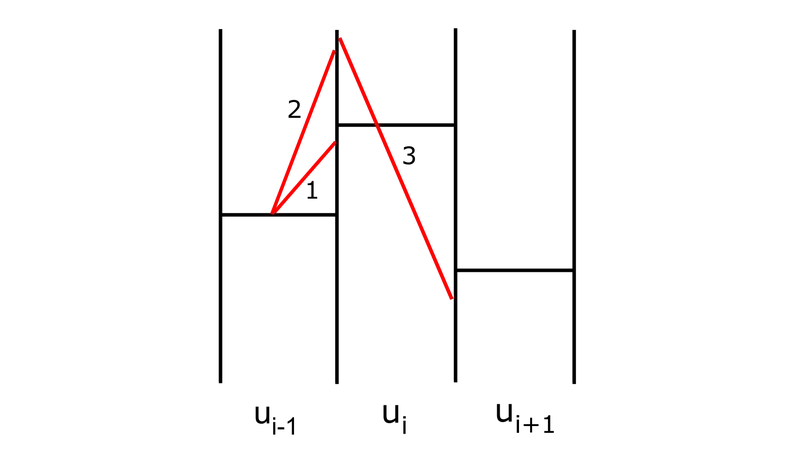Figure 4

The idea is to address the source of the oscillation, i.e. the extrapolation. In Figure 4, we see for extrapolation (1) `u_(i-1)` that the gradient is lower than the cell average of `u_i`, then a new maximum is not created. However, if the gradient is large enough that the extrapolation (2) goes beyond the cell average of the next cell, then a new maximum is created. Similarly, if the gradient is negative, the extrapolation (3) would overshoot the next cell `u_(i+1)` value, and a new minimum is potentially created. So, whenever a large gradient is computed that causes the extrapolation to overshoot the next cell value, then, a 'limit' should be put on the gradient.