A comparison of the rate of convergence for the steady-state and transient-state of 2-D heat conduction equation using Matlab
AIM: To compare the convergence rate (number of iterations) of the steady-state and transient (unsteady)-state heat conduction analysis using Matlab
GIVEN: Top Boundary = 600 K; Bottom Boundary = 900 K; Left Boundary = 400 K; Right Boundary = 800 K; Absolute error criteria = 1e-4
THEORY:
(This is explained in the project 'Solving the steady and unsteady 2-D heat conduction equation using Matlab'. However, the important equations will be stated here for reference.)
The 2D transient heat conduction equation is given as-
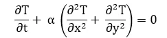
Steady-state and Transient (unsteady) state
- Steady-state Analysis
For steady-state, the equation is-
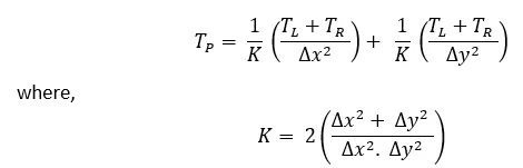
- Transient or Unsteady-state Analysis
The equation is -

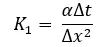

CODE:
Assumptions-
- The domain is a unit square, L = 1
- An equal number of nodes in x and y, nx = ny
- error = 9e9
- Relaxataion factor, omega = 1.1
- Co-efficient of thermal diffusion, alpha = 1.4
(A few changes are made to the code compared to the previous challenge to plot the 3 outputs together)
1. Steady-state Analysis
clear all
close all
clc

L = 1; %Length of the Domain
nx = 50; %Nodes
omega = 1.1;
error = 9e9;
error1=error;error2=error;error3=error;

tol = 1e-4;
ct1 = 0; ct2=0; ct3=0;
ny=nx;
x=linspace(0,L,nx);
dx=x(2)-x(1);
y=linspace(0,L,ny);
dy=y(2)-y(1);

T=300*ones(nx,ny);
T(:,1)= 400 ; %Left Wall
T(1,:)= 600; %Top Wall
T(:,end)= 800; %Right Wall
T(end,:)= 900; %Bottom Wall

T(1,1)= (400+600)/2 ;
T(1,end)= (600+800)/2 ;
T(end,1)= (400+900)/2 ;
T(end,end)= (900+800)/2 ;

T1 = T; T2 = T; T3=T;
Told1 = T1; Told2 = T2; Told3=T;

k = 2*((dx^2+dy^2)/(dx^2*dy^2));

% Jacobi-solver
    tic
    while(error1>tol)
        % Space Loop
        for i = 2:nx-1
            for j = 2:ny-1
                H1 = ((Told1(i-1,j)+ Told1(i+1,j))/(k*dx^2));
                V1 = ((Told1(i,j-1)+ Told1(i,j+1))/(k*dy^2));
                T1(i,j) = H1+V1;
            end
        end
        error1 = max(max(abs(Told1 - T1)));
        Told1 = T1;
        ct1 = ct1 + 1;
    end
    time1 = toc;

% Gauss-Seidel solver
    tic
    while(error2>tol)
        % Space Loop
        for i = 2:nx-1
            for j = 2:ny-1
                H2 = ((T2(i-1,j)+ Told2(i+1,j))/(k*dx^2));
                V2 = ((T2(i,j-1)+ Told2(i,j+1))/(k*dy^2));
                T2(i,j) = H2+V2;
            end
        end
        error2 = max(max(abs(Told2 - T2)));
        Told2 = T2;
        ct2 = ct2 + 1;
    end
    time2 = toc;

% SOR Solver
    tic
    while(error3>tol)
        % Space Loop
        for i = 2:nx-1
            for j = 2:ny-1
                H3 = ((T3(i-1,j)+ Told3(i+1,j))/(k*dx^2));
                V3 = ((T3(i,j-1)+ Told3(i,j+1))/(k*dy^2));
                T3(i,j) = (1-omega)*(Told3(i,j)) + (omega*(H3 + V3));
            end
        end
        error3 = max(max(abs(Told3 - T3)));
        Told3 = T3;
        ct3 = ct3 + 1;
    end
    time3 = toc;

% Plotting
p1 = [.4 .685 .2 .2];
subplot('Position',p1);
contourf(x,y,T1,'ShowText','on');
colorbar
colormap(jet)
xlabel('X-axis');
ylabel('Y-axis');
xticks([0 0.5 1])
text = sprintf('Steady-state heat conduction analysis using iterative solvers nn Method: Jacobi, No of iterations= %d, Time: %f s',ct1 ,time1);
title(text);
set(gca,'YDIR','reverse');

p2 = [.4 .38 .2 .2];
subplot('Position',p2);
contourf(x,y,T2,'ShowText','on');
colorbar
colormap(jet)
xlabel('X-axis');
ylabel('Y-axis');
xticks([0 0.5 1])
text = sprintf('Method: Gauss-Seidel, No of iterations= %d,  Time: %f s',ct2 ,time2);
title(text);
set(gca,'YDIR','reverse');

p3 = [.4 .07 .2 .2];
subplot('Position',p3);
contourf(x,y,T3,'ShowText','on');
colorbar
colormap(jet)
xlabel('X-axis');
ylabel('Y-axis');
xticks([0 0.5 1])
text = sprintf('Method: SOR, No of iterations= %d, Time: %f s',ct3 ,time3);
title(text);
set(gca,'YDIR','reverse');

%xxxxxxxxxxxxxxxxxxxxxxxxxxxxxxxxxxxxxxxxxxxxxxxxxxxxxxxxxxxxxxxxxxxxxxxxxxxxxxxxxxxxxxxxxxxxxxxxxxxxxxxx%
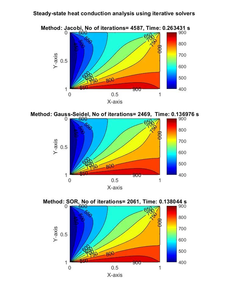
OUTPUT:
2.1 Transient analysis (Implicit)
clear all
close all
clc

L = 1; %Length of the Domain
nx = 50; %Nodes
ny=nx;

x=linspace(0,L,nx);
dx=x(2)-x(1);
y=linspace(0,L,ny);
dy=y(2)-y(1);
t = 0.1;
nt = 1400;
dt = t/nt;
omega  = 1.1;
alpha = 1.4;
ct = 0;
ct1 = 0; ct2=0; ct3=0;
error = 9e9;
error1=error;error2=error;error3=error;
tol = 1e-4;

T=300*ones(nx,ny);
T(:,1)= 400 ; %Left Wall
T(1,:)= 600; %Top Wall
T(:,end)= 800; %Right Wall
T(end,:)= 900; %Bottom Wall

T(1,1)= (400+600)/2 ;
T(1,end)= (600+800)/2 ;
T(end,1)= (400+900)/2 ;
T(end,end)= (900+800)/2 ;

T1 = T; T2 = T; T3=T;
Told1 = T1; Told2 = T2; Told3=T;

T_prev1 = T1; T_prev2 = T2;T_prev3 = T3;
k1 = (alpha*dt)/(dx^2);
k1_1=k1;k1_2=k1;k1_3=k1;
k2 = (alpha*dt)/(dy^2);
k2_1 =k2;k2_2 =k2;k2_3 =k2;


%prompt = 'Choose any one of the options and press Enter nChoose iterative solver type, 1 = Jacobi solver, 2 = GS Solver, 3 = SOR method n';
%iterative_solver = input(prompt);
%if iterative_solver == 1


    tic
    %Jacobi = 1;
    for k = 1:nt
        error1 = 9e9;
        while(error1>tol)
            for i = 2:nx-1
                for j =2:ny-1
                    term1_1 = 1/(1+2*k1_1+2*k2_1);
                    term2_1 = k1_1*term1_1;
                    term3_1 = k2_1*term1_1;
                    H1 = (Told1(i-1,j) + Told1(i+1,j));
                    V1 = (Told1(i,j+1) + Told1(i,j-1));
                    T1(i,j) = (term1_1*(T_prev1(i,j)))+(term2_1*H1)+(term3_1*V1);
                end
            end
            error1 = max(max(abs(Told1-T1)));
            Told1 = T1;
            ct1 = ct1+1;
        end
        T_prev1 = T1;
    end
    time1 = toc;

%if iterative_solver == 2
    tic
    %GS = 2;
    for k = 1:nt
        error2 = 9e9;
        while(error2>tol)
            for i = 2:nx-1
                for j =2:ny-1
                    term1_2 = 1/(1+2*k1_2+2*k2_2);
                    term2_2 = k1_2*term1_2;
                    term3_2 = k2_2*term1_2;
                    H2 = (T2(i-1,j) + Told2(i+1,j));
                    V2 = (Told2(i,j+1) + T2(i,j-1));
                    T2(i,j) = (term1_2*(T_prev2(i,j)))+(term2_2*H2)+(term3_2*V2);
                end
            end
            error2 = max(max(abs(Told2-T2)));
            Told2 = T2;
            ct2 = ct2+1;
        end
        T_prev2 = T2;
    end
    time2 = toc;


%if iterative_solver == 3
    tic
    %SOR = 3;
    for k = 1:nt
        error3 = 9e9;
        while(error3>tol)
            for i = 2:nx-1
                for j =2:ny-1
                    term1_3 = 1/(1+2*k1_3+2*k2_3);
                    term2_3 = k1_3*term1_3;
                    term3_3 = k2_3*term1_3;
                    H3 = (T3(i-1,j) + Told3(i+1,j));
                    V3 = (Told3(i,j+1) + T3(i,j-1));
                    T3(i,j) = (1-omega)*(Told3(i,j)) + (omega*((term1_3*(T_prev3(i,j)))+(term2_3*H3)+(term3_3*V3)));
                end
            end
            error3 = max(max(abs(Told3-T3)));
            Told3 = T3;
            ct3 = ct3+1;
        end
        T_prev3 = T3;
    end
    time3 = toc;

p1 = [.4 .685 .2 .2];
subplot('Position',p1);
contourf(x,y,T1,'ShowText','on');
colorbar
colormap(jet)
xlabel('X-axis');
ylabel('Y-axis');
xticks([0 0.5 1])
text = sprintf('Transient/unsteady-state heat conduction analysis using iterative solvers nn Method: Jacobi, No of iterations= %d, Time: %f s',ct1 ,time1);
title(text);
set(gca,'YDIR','reverse');

p2 = [.4 .38 .2 .2];
subplot('Position',p2);
contourf(x,y,T2,'ShowText','on');
colorbar
colormap(jet)
xlabel('X-axis');
ylabel('Y-axis');
xticks([0 0.5 1])
text = sprintf('Method: Gauss-Seidel, No of iterations= %d,  Time: %f s',ct2 ,time2);
title(text);
set(gca,'YDIR','reverse');

p3 = [.4 .07 .2 .2];
subplot('Position',p3);
contourf(x,y,T3,'ShowText','on');
colorbar
colormap(jet)
xlabel('X-axis');
ylabel('Y-axis');
xticks([0 0.5 1])
text = sprintf('Method: SOR, No of iterations= %d, Time: %f s',ct3 ,time3);
title(text);
set(gca,'YDIR','reverse');
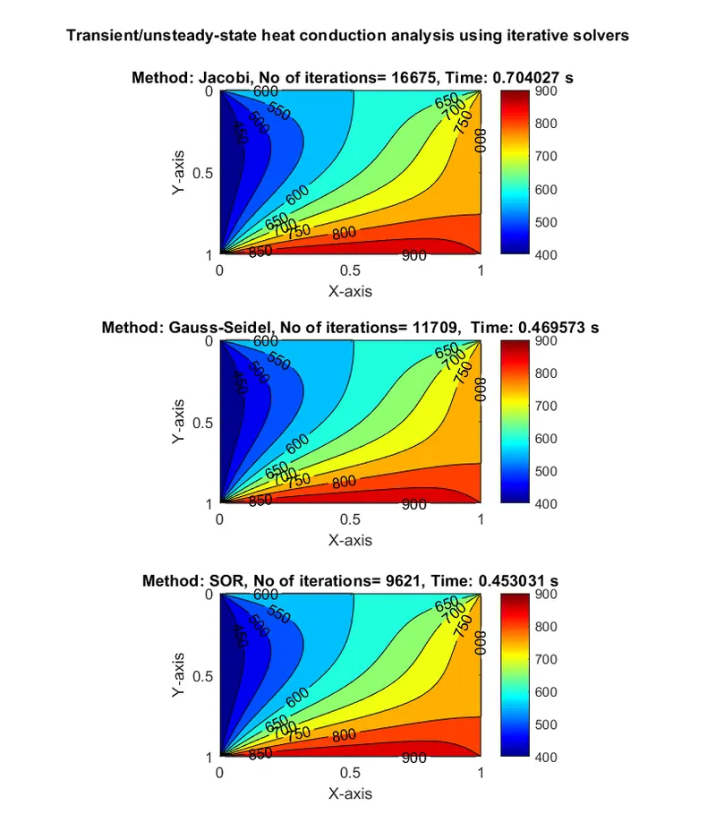
OUTPUT:
2.2 Transient analysis (Explicit)
clear all
close all
clc

L = 1; %Length of the Domain
nx = 50; %Nodes
ny=nx;

x=linspace(0,L,nx);
dx=x(2)-x(1);
y=linspace(0,L,ny);
dy=y(2)-y(1);
t = 0.1;
nt = 1400;
dt = t/nt;
alpha = 1.4;
CFL_x= alpha*dt/(dx)^2;
CFL_y= alpha*dt/(dy)^2;
ct = 0;

T=300*ones(nx,ny);
T(:,1)= 400 ; %Left Wall
T(1,:)= 600; %Top Wall
T(:,end)= 800; %Right Wall
T(end,:)= 900; %Bottom Wall

T(1,1)= (400+600)/2 ;
T(1,end)= (600+800)/2 ;
T(end,1)= (400+900)/2 ;
T(end,end)= (900+800)/2 ;

Told = T;
k1 = (alpha*dt)/(dx^2);
k2 = (alpha*dt)/(dy^2);

tic
for k = 1:nt
    for i = 2:nx-1
        for j =2:ny-1
            H = (Told(i-1,j) - 2*Told(i,j) + Told(i+1,j));
            V = (Told(i,j+1) - 2*Told(i,j) + Told(i,j-1));
            T(i,j) = Told(i,j) + k1*H + k2*V;
        end
    end
    Told = T;
    ct = ct+1;
    time = toc;
end
figure(1)
contourf(x,y,T,'ShowText','on');
colorbar
colormap(jet)
xlabel('x');
ylabel('y');
text = sprintf(' Transient/unsteady-state heat conduction analysis (Explicit)n Method: Explicit, No.of Iterations: %d, Time reqd.: %f',ct, time );
title(text);
set(gca,'YDIR','reverse');
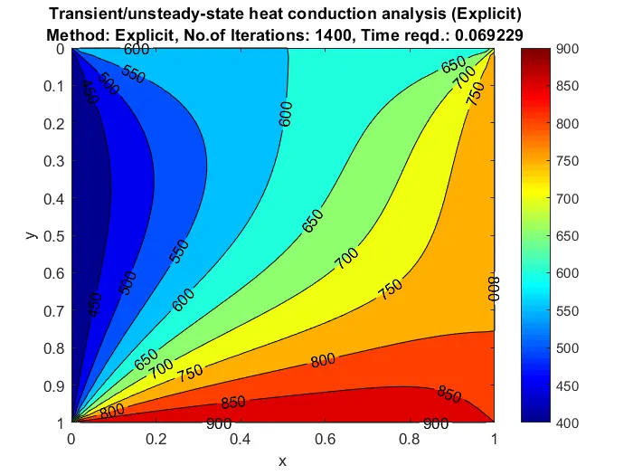
OUTPUT:
SUMMARY:
1. First of all, with regard to the rate of convergence, it can be observed that the sequence for the number of iterations required is as follows- Jacobi > Gauss-Seidel > SOR.
In the Jacobi method, to calculate TP, we use the older values for TL, TR, TB, and TT from the previous iteration. However, in the Gauss-Seidel method, TL and TB are already known and hence the new updated values are used every time. This leads to a significant decrease in the number of iterations required for convergence. SOR method is an updated form of the Gauss-Seidel method wherein the use of an optimal value (say 1.1, over-relaxation) of the relaxation factor 'omega' leads to faster convergence and a lesser number of iterations.
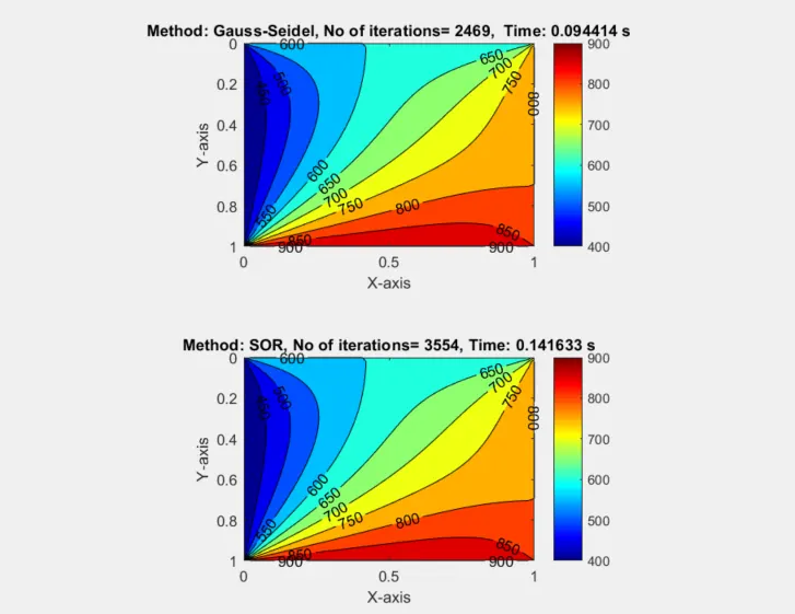
However, when the value of omega < 1 (under-relaxation), it can lead to an increase in the number of iterations (see figure below, omega = 0.8) as compared to the Gauss-Seidel method.
2. The number of iterations required for the Transient analysis is higher than the steady analysis.
This is because in transient cases, the convergence loop is within a time-loop. This means that after each time-step, the temperature T is used in the next time-step as the new temperature T, and the whole process is repeated for the given number of time-steps. Thus, the number of iterations is increased significantly.
In the explicit case, no iterative solvers are required as all the terms on the RHS are known and the convergence is attained using a time-marching approach and an optimal number of time-steps.