Week 9 - FVM Literature Review
Finite Volume Method (FVM):
The finite volume method is a method for representing and evaluating partial differencing equations in the form of algebraic equations. In the finite volume method, volume integrals in a partial differential equation that contain a divergence term are converted to surface integrals, using the divergence theorem. These terms are evaluated as fluxes at the surface of each finite volume. Because the flux entering a given volume is identical to that leaving the adjacent volume, these methods are conservative. Another advantage of the finite volume method is that it is easily formulated to allow for unstructured meshes. The method is used in many CFD packages. The control volume integration, which forms a key step of the FVM.
Consider steady-state heat diffusion of property T in the 1D domain defined in the below figure:
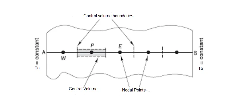
From the above figure, p is the general nodal point and the nodes to the west and east, are identified by W and E respectively. The west side face of the control volume is referred to by w and the east side control volume face by e.
The finite volume refers to the small volume surrounding each node point. FVM can be compared and contrasted with the FDM, which approximate derivatives using nodal values, or finite element method, which create local approximations of a solution using local data, and construct a global approximation by stitching them together. In contrast, a finite volume method evaluates exact expressions for the average value of the solution over some volume and uses this data to construct approximations of the solution within cells.
Interpolation schemes:
The approximation of surface and volume integrals may require values of the variable at locations other than the computational nodes of the control volume. Values at these locations are obtained using the interpolation formula. There are different interpolation schemes, they are as follows:
1. Upwind Interpolation:
The upwind interpolation for approximating the value of a variable at the east face of the control volume is given by
`f_e` = `f_p` if `(v*n)_e > 0` ; `f_e` if `(v*n)_e < 0`
This interpolation scheme is equivalent to using a backward or forward finite difference approximation(depending on the flow direction).
2. Linear Interpolation or Central difference Interpolation(CDS):
The approximation value of the variable at the control volume face center by linear interpolation of the values at two nearest computational nodes.
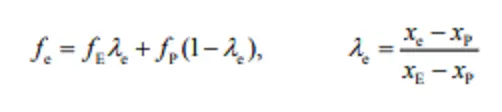
The linear interpolation is equivalent to the use of the central difference formula of the first-order derivative, and hence, this scheme is also termed as central differencing schemes(CDS). This scheme is second-order accurate and may produce oscillatory solutions.
3. Quadratic upwind differencing interpolation(QUICK):
QUICK stands for the Quadratic upwind Interpolation for Convective Kinetics scheme of Leonard(1979) uses a three-point upstream-weighted quadratic interpolation for cell face values. It approximates the values of the variable at the control volume face center by quadratic interpolation of the values at three nearest computational nodes(one downstream node D and two upstream nodes U and UU).
`g_1 = ((x_e-x_U)*(x_e-x_(UU)))/((x_(UU)-x_U)(x_(UU)-x_D))`
`g_2= ((x_e-x_U)*(x_e-x_(D)))/((x_(UU-x_U))*(x_(UU)-x_D))`
Flux Limiters:
The convective fluid flow it has been observed that low order schemes are usually stable but quite dissipative in nature around points of discontinuity while the higher-order schemes are unstable in nature. Highly accurate and oscillation free schemes are known as High-resolution schemes. They are used in high-resolution schemes for solving problems described by PDEs.
Flux limiter functions are used to tune high order and low order schemes in such a way that the resulting scheme gives a high order accuracy in the smooth region of the flow and maintains 1st order accuracy in the vicinity of shocks.
Consider the 1D semi-discrete scheme below,

in the above equation, `F(u_(i+1/2))` and `F(u_(i-1/2))` represented by low and high-resolution schemes, then the flux limiter can switch between these schemes depending upon the gradients close to the particular cell as follows,
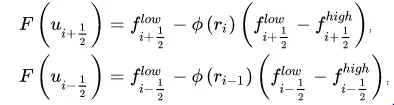
where,
`f^(flow)` = low resolution flux,
`f^(high)` = high resolution flux,
`phi(r)` = flux limiter function, and r represents the ratio of successive gradients on the solution mesh, i.e,
`r_i` = `(u_i -u_(i-1))/(u_(i+1)-u_i)`
The limiter function is constrained to be greater than or equal to 0, i.e., `phi(r) >= 0`. Therefore, when the limiter is equal to zero, the flux represented by a low-resolution scheme, and the limiter is equal to 1, the flux represented by a high-resolution scheme. The common forms of flux limiter functions: CHARM, HCUS, Koren, HQUICK, etc.
Example:
The FVM to the solution of a simple diffusion problem involving conductive heat transfer is presented here. The 1D steady-state conductive heat transfer is given below:
`d/dx*(k(dt)/(dx))+S = 0`
In the above equation, k indicates thermal conductivity and the independent variable is temperature T. S is the source term.