Week 9 - FVM Literature Review
What is the Finite Volume Method(FVM) ?
The Finite Volume Method (FVM) is a discretization method for the approximation of a single or a system of partial differential equations expressing the conservation, or balance, of one or more quantities. These partial differential equations (PDEs) are often called conservation laws; they may be of different nature, e.g. elliptic, parabolic or hyperbolic, and they are used as models in a wide number of fields, including physics, biophysics, chemistry, image processing, finance, dynamic reliability. They describe the relations between partial derivatives of unknown fields such as temperature, concentration, pressure, molar fraction, the density of electrons, or probability density function, with respect to variables within the domain (space, time,...) under consideration.
As in the finite element method, a mesh is constructed, which consists of a partition of the domain where the space variable lives. The elements of the mesh are called control volumes. The integration of the PDE over each control volume results in a balance equation. The set of balance equations is then discretized with respect to a set of discrete unknowns. The main issue is the discretization of the fluxes at the boundaries of each control volume: in order for the FVM to be efficient, the numerical fluxes are generally
conservative, i.e. the flux entering a control volume from its neighbor must be the opposite of the one entering the neighbor from the control volume,
consistent, i.e. the numerical flux of a regular function interpolation tends to the continuous flux as the mesh size vanishes.
It is sometimes possible to discretize the fluxes at the boundaries of the control volume by the finite difference method (FDM). In this case, the method has often been referred to as a finite difference method or conservative finite difference method. The specificity of the FVM with respect to the FDM is that the discretization is performed on the local balance equations, rather than the PDE: the fluxes on boundaries of the control volumes are discretized, rather than the continuous differential operator.
The resulting system of discrete equations depends on a discrete (finite) set of unknowns, and may be either linear or non-linear, depending on the original problem itself; this system is then solved exactly or approximately, using for example direct or iterative solvers in the case of linear equations and fixed point or Newton-type methods in the case of nonlinear equations.
Let us emphasize that there is no systematic way to derive the discrete system from the continuous one; in fact, the physical or engineering knowledge of the problem is in many cases the key ingredient in order to obtain a scheme that satisfies the expected properties of accuracy, robustness, and computational cost. Let us mention that in some cases, the engineering problem is initially set at a discrete level: the model consists of a set of discrete balance equations and is therefore written as a finite volume scheme, and the continuous model of the problem is not explicitly given.
Many of these issues have often been addressed in computational fluid mechanics. A review of the schemes for the discretization of the compressible and incompressible Navier-Stokes and Euler equations may be found in e.g. Wesseling 2001, Feistauer et al. 2003. The FVM has also been very early introduced in the framework of oil reservoir engineering.
write down the major differences between FDM & FVM ?
Finite-Difference Method: Advantages and Disadvantages
The finite-difference method is defined dimension per dimension; this makes it easy to increase the “element order” to get higher-order accuracy. If you can fit the simulation in a rectangular or box-shaped geometry using a regular grid, efficient implementations are much easier than for finite-element and finite-volume methods. Regular grids are useful for very-large-scale simulations on supercomputers often used in, as mentioned before, meteorological, seismological, and astrophysical simulations.
With the finite-difference method, you may easily run into problems handling curved boundaries for the purpose of defining the boundary conditions. Boundary conditions are needed to truncate the computational domain. They represent communication with the surrounding world, which is the part that you do not want to be included in your simulation. If one can overcome the boundary-condition problem on curved boundaries, the method gives very efficient and high-quality results.
For computations that need high accuracy, the extra effort in making boundary-fitted meshes and the associated complications of such meshes for the implementation may be worth it. Examples include Formula 1 car computational-fluid-dynamic (CFD) simulations and space-shuttle CFD simulations. The finite-difference method is more difficult to use for handling material discontinuities. In addition, it does not lend itself to local grid refinement or anything similar to “adaptive mesh refinement.” This may be needed to resolve local rapid variations in solutions such as around a corner of a complex shape, as described earlier.
Finite-Volume Method: Advantages and Disadvantages
The finite-volume method is a natural choice for CFD problems since the partial differential equations you have to solve for CFD are conservation laws. However, both finite differences and finite elements can also be used for CFD. Efficient technology for CFD with the finite-element method has become increasingly popular over the last 10 to 15 years. Techniques for CFD with the finite-difference and finite-volume method have been known and used much longer.
The finite-volume method’s strength is that it only needs to do flux evaluation for the cell boundaries. This also holds for nonlinear problems, which makes it extra powerful for robust handling of (nonlinear) conservation laws appearing in transport problems.
The local accuracy of the finite-volume method, such as close to a corner of interest, can be increased by refining the mesh around that corner, similar to the finite-element method. However, the functions that approximate the solution when using the finite-volume method cannot be easily made of higher order. This is a disadvantage of the finite-volume method compared to the finite-element and finite-difference methods.
Difference between FVM & FDM
| FDM | FVM | |
|
|
Need for Interpolation schemes and flux limiters in FVM
- The Guass or divergence theorem simply states that the outward flux of a vector field through a closed surface is equal to the volume integral of the divergence over the region inside the surface.
- This theorem is fundamental in the FVM, it is used to convert the volume integrals appearing in the governing equation into surface integrals.
- The face values appearing in the convective and diffusive fluxes have to be computed by some form of interpolation from the centroid values of the control volume at both sides of the face.
- After spacial discretization, we can proceed with temporal discretization. By proceeding in this way we are using the method of lines (MOL).
- The main advantage of the MOL method is that it allows us to select numerical approximations of different accuracy for the spatial and temporal terms. Each term can be treated differently to yield different accuracies.
- Nearly all flows in nature and industrial applications are unsteady (also known as transient or time-dependent).
- Unsteadiness is due to-
- Instabilities
- Non-equilibrium initial conditions
- Time-dependent boundary conditions
- source term
- chemical reactions
- moving or deforming bodies
- turbulence
- Buoyancy
- Convection
- Multiple phases
Steady Simulation vs Unsteady Simulations:
- Steady simulations require less computational power than unsteady simulations.
- They are also many fasters than unsteady simulations.
- But sometimes they do not converge on the right solution.
- They are easier to post-process and analyze.
- We can use the solution of an unconverted steady simulation as initial conditions for an unsteady simulation.
- Remember, steady simulations are not time accurate, therefore we can not use them to compute temporal statistics or compute the shedding frequency.
1D Linear Heat conduction equation to demonstrate FVM, interpolation, and flux limiter
1D heat conduction equation
`( ∂ /(∂ X )) α . ( (∂ T)/( ∂ X) ) + S = 0`
S is source term which is responsible for heat generation
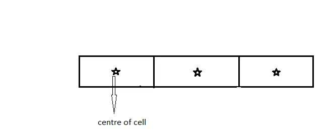
Take three control volume, points inside volume acts as the center of the volume, and PDE is solved for complete volume using surface integral
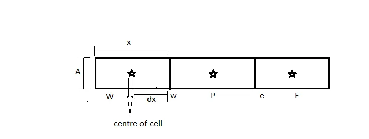
In the above three cells center cell is p and the east and west cells are E & W. w & e act as junctions between these three cells. At e & w interpolation schemes are used.
`∫ ∂/( ∂ X) ( α . (∂ T)/( ∂ X) ) d V + ∫ S d V = 0`
`∫ ∂ /(∂ X) ( α .( ∂ T)/( ∂ X )) A dx + ∫ S d V = 0`
`[(α A ∂ T)/(∂ _x) ] + ∫ S d V = 0`
`∫ S . d V =overlineS . d V`
Now,
`α e [ (A ∂T)/( ∂ Xe) ] − α w [ (A ∂ T)/( ∂ X w) ] + overline S d V = 0`
`α A [(Te −Tp)/(△x)] − α A [(Tp − T w)/(△x)] + overlineS . d V = 0`
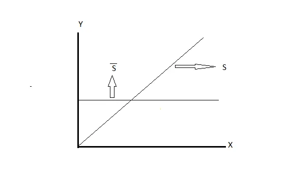
In the above graph linear straight line S is the source term which is varying at a constant slope. `overlineS` is the average of S as S.dv is an area under the curve
So now,
`α A [(Te−Tp)/(△ x) ] − αA [(Tp−Tw)/(△x) ] + S u + S pT p = 0`
The above equation shows that FVM methods are conservative in nature. The total heat of the system sums up to 0.