Week 9 - FVM Literature Review

Objective :

In this challenge we need to adress and answer four major quaestions,what is FVM, dfferences between FDM and FVM, need for interpolation schemes and flux limiters

Theory :

Here we shall try to answer all the four questions one by one respectively

1. FVM : The finite volume method (FVM) is a method for representing and evaluating partial differential equations in the form of algebraic equations. In the finite volume method, volume integrals in a partial differential equation that contain a divergence term are converted to surface intervals, using the divergence theorem. These terms are then evaluated as fluxes at the surfaces of each finite volume. Because the flux entering a given volume is identical to that leaving the adjacent volume, these methods are conservative. Another advantage of the finite volume method is that it is easily formulated to allow for unstructured meshes. The method is used in many CFD(computaional fluid dynamics) packages. "Finite volume" refers to the small volume surrounding each node point on a mesh. In FVM, the domain is made up of arbitrary control volumes (internal and boundary), solution sought in each of the volumes are stored in the cell centroids.

2. Differences between FDM and FVM

FDM : Governing equations are in the differential form , solution computed at each node i.e; intersection of mesh lines , it requires the use of structured grid, difficult to impliment for complex geometrices, easy to obtain higher order schemes, so prefferable for applications that requires very high accuracy, all flow variables need to be differentiable and continuous over entire domain,unsuitable for handling discontinuities also it does not ensure conservation.

FVM : Governing equations are in the integral form, solution computed at the cell centroids, it can handle unstructured grid and hence complex geometrices with ease, deriving schemes higher than second order is next to impossible due to complexity involved, can handle discontinuities due to the nature of integral euations, imposes and ensures conservation at both cell and domain levels

3. Interpolation schemes

It is needed for the evaluation of fluxes at face centres from cell centroids,

Some of the interpolation schemes used are upwind, linear, linearupwind, quadratic ,etc interpolation schemes.

These methods are used toget to more realistic results as the engineering problems basically uses the real world environment.Here in FVM the use of volume instead of a point makes that close to real problems and governing equation needs to be solved for that.

Interpolation Methods in FVM:

Various possibilities for interpolation-

• Upwind Interpolation Scheme
• Linear Interpolation Scheme
• Quadratic upwind Interpolation Scheme
• Hybrid,TVD and ENO Interpolation Scheme

here for example we shall see one or two schemes to get an idea of this whole methods

Upwind Interpolation Scheme -

> It is mainsly used for the convection dominant problems. Velocity for a given point ,the direction of that particular velocity that determines the variables values used in interpolation process. In upwind scheme it make use of nodes that are in the upstream of the given node.

> It is used to calculate the approximate value of the variable(f) at the east face of the control volume, the equation is given by;

> This scheme is almost similar to the forward difference approximation or a backward difference approximation based on the flow direction.

> We know that, when calculating gradience, we need to have those values bounded, so that they dont jump. Hence this approximation satisfies the boundness condition.

Linear Interpolation Scheme -

> Linear interpolation is the method of generating new data points with a range of a discrete set of known data points.

Where,

> The linear Interpolation scheme is same as the central difference formula that we considered for the first order derivative. So this scheme is also known as the central difference scheme.

> Generally it is used to solve the integrated convection-diffusion equation.

> It leads to a easy approximation for the evaluation of gradients that are required for evaluation of diffusive fluxes.

> CDS is a second order accurate and may produce oscillatory solutions i.e here if the grid spacing is very large we can find oscillatory solutions. It is bascially a first order, as we refine the grid then accuracy is close to the second order.

4. Flux limiters :

Most of us might have seen the behaviour of numerical schemes in order to capture shocks and discontinuity that arises in hyperbolic equations. Physically, these equations model the convective fluid flow. It has been observed that low-order schemes are usually stable but quite dissipative in nature around the points of discontinuity/shocks. On the other hand higher-order numerical schemes are unstable in nature and show oscillations in the vicinity of discontinuity. One can have a better understanding of such behaviour by analysing the modified equation of these schemes.

Now as said above one can not have high order accuracy without oscillations. The objective is to have highly accurate and stable oscillation free schemes. This kind of schemes are known as high resolution schemes. In 1984 Harten proposed the constuction and gave TVD criteria for such scheme. Here we talk only about using flux limiters function to construct high resolution schemes. The idea is to tune the numerical flux of high order and low order scheme using the flux limiter function in such a way that the resulting scheme gives a high order accuracy in the smooth region of flow and sticks with first order of accuracy in the vicinity of socks/discontinuities as follows:

Define the numerical flux fuction of high resolution conservative scheme as

where are the numerical flux of conservative low order and high order schemes respectively. and is a function of smoothness parameter usually defined as

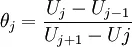
What remains next is to define the limiter fuction in such a way that it satisfies at least the following properties:

• remains positive ,
• satisfies
• passes through a perticular region known as TVD region associted with the underlying scheme in order to guarantee stability of the scheme.