Week 7 - Simulation of a 1D Super-sonic nozzle flow simulation using Macormack Method
Objective: In this challenge we need to simulate the isentropic flow through a quasi 1D subsonic and siper sonic nozzle for both the conservative and non conservative forms of governing equations (continuity, momemtum, energy) by using maccormack method of discretization and to compare the resulsts of both the forms
Theory: A transient isentropic invisid adiabatic compressible flow will be modelled for quasi 1D nozzle chamber, here we nned to understand all the adjectives that define what kind of a flow it is,
firstly the flow is transient which means, it is varrying with respect time,
isentropic = flow has constant entropy, adiabatic = no heat transfer into or out of the system
invsid = zero or negligible viscosity, compressible = flow can experience a density change during flow
this type of flow is modelled for quasi 1D nozzle means that the flow is varrying only in one direction not in 2 or 3 directions
Here after knowing what kind of flow we are simulating we need to know about the nozzle chamber
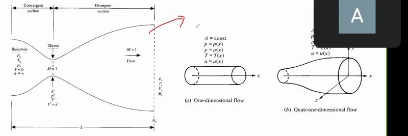 This picture depicts the nozzle chamber
as shown in the image nozzle has convergent section wher the flow is converged and the throat section where flow is compressed and the divergent section where flow is divereged hence more velocity fluid will be outflowed , The flow variables through the nozzle chambers are pressure, density, velocity, area and temparature.
mach number = ratio of object speed to the speed of sound in the medium which object travels
here if mach number M>=0.3 then the fluid is said to be compressible , if M<0.3 then fluid is said to incompressible
Here convergent section is calles as subsonic section as the mach number will be less than one M<1
throat section is sonic mach number is one M=1 and divergent section is supersonic as mach number is greater than one M>1
Here intially flow converges in convergent section where pressure is high and the velocity is low, at throat section flow will get choked also as cross sectional area becomes smaller fluid experiences a pressure drop as it exits from the other end of nozzle but velocity increases considerable as it expands in the divergent section
Now we shall see the Governing equations for this type of flow which is euler equations ,
drhoA/dt + drhoAu/dx =0
rhodu/dt + rhoudu/dx = -drho/dx
rhode/dt + rhoude/dx = -pdu/dx - pudlnA/dx
The PDE type will be for unsteady euler equations is governed by hyberbolic behaviour for subsonic and supersonoc nozzle regimes , where as steady euler equations is elliptical in nature in subsonic region and hyperbolic nature in supersonic region ,
Now we shall see the how we obtain both conservative and non conservative forms by deriving from the above mentioned governing equations one by one
By deriving and simplifying the the governing equations we get non-conservative form and conservative form which is given below
1. Non-conservative form : governing equations
A) continuity = drho'/dt' = -rho'dv'/dx' -rho'v'd(lnA')/dx' -v'drho'/dx'
B) momemtum = dv'/dt' = -v'dv'/dx' - 1/gamma*(dT'/dx' + T'/rho'*drho'/dx')
C) energy = dT'/dt' = -v'dT'/dx' -(gamma-1)*T'(dv'/dx' + v'*d(lnA')/dx').
where T' = T/T0 , rho' = rho/rho0 , x' = x/L, v' = v/a0, A' = A/A*, t' = t/L/a0 these are all the non dimensionalised variables
2. conservative forms : governing equations
A) continuity = d(rho'A')/dt' + d(rho'*A'*v')/dx' = 0
B) momentum = d(rho'*A'*v')/dt' + d(rho'*A'*v'^2 + (1/gamma)*rho'*A'/dx' = 1/gamma*p'*dA'/dx'
C) energy = d(rho'*(e'/gamma-1 + gamma/2v'^2)*A')/dt' + d(rho'(e'/gamma-1 + gamma/2*v'^2)*v'*A' + p'*A'*v')/dx' = 0
where u1 = rho'*A', u2 = rho'*A'*v' , u3 = rho'(e'/gamma-1 + gamma/2*v'^2)*A',
F1 = rho'*A'*v', F2 = rho'A'*v'^2 + 1/gamma*p'*A', F3 = rho'(e'/gamma-1 + gamm/2*v'^2)*v'*A' + p'*A'*v'
J2 = 1/gamma*p'*dA'/dx'
Now to solve this equations first we need to create one dimensioned grid then we use the unique discretization technique called maccormack method and then apply initial and boundary conditions
Discretization scheme = Maccormack method
here we use time marching solutions,in which we take the values of previous tme step and compute the next time step and go on until we get actual value.
Maccormack method is also a time marching solution but we split it into two 1. predictor step and 2. corrector step. first we take the initial condition values and apply predictor step to find the next time step values after that we update the solution obtained from the predictor step and apply corrector step by giving the updated values , then we compute the average time derivatives by taking corrector step values after which the actual values are computed easily in the next time step.
Here the main difference between predictor and corrector step is that predictor step uses FDS(forward differencing scheme), corrector step uses BDS (backward differencing scheme), for space terms i:e (RHS side governing equations)
Now we shall apply maccormack method to the governing equations(continuity, momemtum, energy) of both conservative and non-conservative forms seperately and derive the equations for both predictor and corrector steps respectively
1. Non-conservative form
A. Predictor step (FDS) forward differncing scheme
a) continuity equation = (drho/dt)'(i) = -rho'(i) * v'(i+1) -v'(i)/dx - rho'(i)*v'(i)*ln A(i+1) - lnA'(i)/dx - v'(i)* (rho'(i+1) - rho'(i)/dx
b) momentum equation = (dv/dt)'(i) = -v'(i)*v'(i+1) - v'(i)/dx - 1/gamma(T'(i+1) - T'(i)/dx + T'(i)/rho'(i)* rho'(i+1) - rho'(i)/dx)
c) energy equation = (dT/dt)'(i) = -v'(i)8(T'(i+1) - T'(i)/dx - (gamma-1)*T'(i)*(v'(i+1) - v'(i)/dx + v'(i)*lnA'(i+1) -lnA'(i)/dx)
B. corrector step (BDS) backward difference scheme
a) continuity equation = (drho/dt)'(i) = -rho'(i) * v'(i) -v'(i-1)/dx - rho'(i)*v'(i)*ln A(i) - lnA'(i-1)/dx - v'(i)* (rho'(i) - rho'(i-1)/dx
b) momentum equation = (dv/dt)'(i) = -v'(i)*v'(i) - v'(i-1)/dx - 1/gamma(T'(i) - T'(i-1)/dx + T'(i)/rho'(i)* rho'(i) - rho'(i-1)/dx)
c) energy equation = (dT/dt)'(i) = -v'(i)8(T'(i) - T'(i-1)/dx - (gamma-1)*T'(i)*(v'(i) - v'(i-1)/dx + v'(i)*lnA'(i) -lnA'(i-1)/dx)
2. conservative form
A. Predictor step (FDS) forward differncing scheme
a) continuity equation = (du1/dt)'(i=16) = -(F1)i=17 - (F1)i=16/dx'
b) momentum equation = (du2/dt)'(i=16) = -(F2)i=17 - (F2)i=16/dx' +J2
c) energy equation = (du3/dt)'(i=16) = -(F3)i=17 - (F3)i=16/dx'
B. corrector step (BDS) backward difference scheme
a) continuity equation = (du1/dt)'(i=16) = -(F1)i=16 - (F1)i=15/dx'
b) momentum equation = (du2/dt)'(i=16) = -(F2)i=16 - (F2)i=15/dx' +J2
c) energy equation = (du3/dt)'(i=16) = -(F3)i=16 - (F3)i=15/dx'
Now we look here that this type of PDE type problem requires initial and boundary conditions, nozzle has both inlet and outlet hence boundary conditions has to be applied for both inlet and outlet regions,
Inlet BC : subsonic region
1) RRC : dirchlet, 2) SD : dirichlet, 3) LRC : neumann
Outlet BC : super sonic region
1) RRC : neumann , 2) SD : neumann , 3) LRC : neumann , here RRC = right running characteric , LRC = left running characteric , SD = stearmline direction
Dirichlet boundary conditions prescribe the numerical value that the variable at the domain boundary should assume like pressure or velocity , neumann boundary conditions assumes the value of derivative of the variable applied at the domain boudary as opposed to the variale itself as in the dirichlet boundary conditions
1.] For conservation form
initial conditions = A = 1+2.2(x-1.5)^2 where 0<_ x <_ L
v = u2/rho*A.
dirichlet and neumann BC's are
inlet u1 = rho1*A1 = 1, u2 = 2u2-2u3, u3 = u1*(T1/gamma-1 + gamma/2 *(u2/u1)^2)
outlet u1 = 2u1(n-1) - u1(n-2), u2 = 2u2(n-1) - u2(n-2), u3 = 2u3(n-1) - u3(n-2)
2.] For non-conservation form
initial conditions = A = 1+ 2.2(x - 1.5)^2, where 0<_x<_L , rho = 1-0.3146x , T = 1- 0.2314x, v= (0.1 - 1.09x)*t/2
dirichlet and neumann BC's are
inlet rho1 =1 , T1 =1, v1 = 2v2-v3
outlet rho(n) = 2rho(n-1)- rho(n-2),
T(n) = 2T(n-1)- T(n-2),
v(n) = 2v(n-1)- v(n-2),
Down here are the programmes of the both conservative and non-conservative forms of governing equations attached using insert code option and the respective plots are attached using insert image option please check it
1. non-conservative form (programme)
In this programme first we give all the neccessary input variables and define them, calculate initial profiles such as pressure,area,velocity,temparature, and then provide the time steps , then create outer time loop give the time step condition and solve the predictor step method by giving the above mentioned equations of maccormack method and update all the values required and then woith the neccessary input condition, apply corrector step method and compute the values for all the variables,and update the values and compute average time derivate ,then apply respective boundary conditions at inlet and the outlet of nozzle provided above and plot for all the varibles with 'x' i:e nozzle length vs pressure,velocity,temparature,density and mach number and do the same with time steps and also plot mass flow rate vs nozzle length , observe the results and plots
clear all
close all
clc

% Inputs
n = 31
x = linspace(0,3,n);
dx = x(2)-x(3);
gamma = 1.4

% Calculate initial profiles

rho = 1-0.3146*x;
t = 1-0.2314*x; % t = temparature
v = (0.1+1.09*x).*t.^0.5;

% area
a = 1+2.2*(x-1.5).^2;

% Time steps
nt = 10;
dt = 0.01;

th = round(n/2);

cfl = (max(v+sqrt(t))*dt/dx);

% Outer time loop
for k = 1:nt

rho_old = rho;
v_old = v;
t_old = t;

   % Predictor method

    for j = 2:n-1
         % drho_dt_p = -rho(j)*(v(j+1)-v(j))/dx - rho(j)*v(j)*(log(a(j+1))-log(a(j)))/dx - v(j)*(rho(j+1)-rho(j))/dx;
         dvdx = (v(j+1)-v(j))/dx;
         drhodx = (rho(j+1)-rho(j))/dx;
         dtdx = (t(j+1)-t(j))/dx;
         dlogadx = (log(a(j+1))-log(a(j)))/dx;

         % continuity equation
         drhodt_p(j) = -rho(j)*dvdx-rho(j)*v(j)*dlogadx - v(j)*drhodx;

         % momemtum equation
         dvdt_p(j) = -v(j)*dvdx - (1/gamma)*(dtdx + (t(j)/rho(j))*drhodx);

        % energy equation
        dtdt_p(j) = -v(j)*dtdx - (gamma-1)*t(j)*(dvdx + v(j)*dlogadx);

       % solution update
       rho(j) = rho(j) + drhodt_p(j)*dt;
       v(j) = v(j) + dvdt_p(j)*dt;
       t(j) = t(j) + dtdt_p(j)*dt;

    end

    % Corrector method

for j = 2:n-1
    % drho_dt_p = -rho(j)*(v(j+1)-v(j))/dx - rho(j)*v(j)*(log(a(j+1))-log(a(j)))/dx - v(j)*(rho(j+1)-rho(j))/dx;
         dvdx = (v(j)-v(j-1))/dx;
         drhodx = (rho(j)-rho(j-1))/dx;
         dtdx = (t(j)-t(j-1))/dx;
         dlogadx = (log(a(j))-log(a(j-1)))/dx;

         % continuity equation
         drhodt_c(j) = -rho(j)*dvdx-rho(j)*v(j)*dlogadx - v(j)*drhodx;

         % momemtum equation
         dvdt_c(j) = -v(j)*dvdx - (1/gamma)*(dtdx + (t(j)/rho(j))*drhodx);

        % energy equation
        dtdt_c(j) = -v(j)*dtdx - (gamma-1)*t(j)*(dvdx + v(j)*dlogadx);


end

% Compute the average time derivative

drhodt = 0.5*(drhodt_p + drhodt_c)
dvdt = 0.5*(dvdt_p + dvdt_c)
dtdt = 0.5*(dtdt_p +dtdt_c)


% Final solution update
  for i = 2:n-1
    rho(i) = rho_old(i) + drhodt(i)*dt
    v(i) = v_old(i)+ dvdt(i)*dt
    t(i) = t_old(i) + dtdt(i)*dt
  end

  % Apply the boundary conditions
  % Inlet
  v(1) = 2*v(2) -v(3);

  % Outlet
  v(n) = 2*v(n-1) - v(n-2);
  rho(n) = 2*rho(n-1) - rho(n-2);
  t(n) = 2*t(n-1) - t(n-2);

  % Pressure
  p = rho.*t;
  % Machnumber
  M = v./sqrt(t);
  % Mass flow rate
  m = rho.*a.*v;

  figure(3)
  hold on
  if k == 1
      plot(x,m);
  end
  if k == 50
      plot(x,m);
  end
  if k == 250
      plot(x,m);
  end
  if k == 500
      plot(x,m);
  end
  if k == 750
      plot(x,m);
  end
  if k == 1200
      plot(x,m);
  end

  rho_throat(k) = rho(th);
  v_throat(k) = v(th);
  t_throat(k) = t(th);
  p_throat(k) = p(th);
  M_throat(k) = M(th);

end
xlabel('nozzle length')
ylabel('mass flow rate')
legend('1dt','50dt','250dt','500dt','750dt','1200dt')
title('variation of mass flow rate at different time steps')


figure(1)
subplot(5,1,1)
plot(x,v)
xlabel('nozzle length')
ylabel('velocity')
title ('steady state primitive variable profiles')
subplot(5,1,2)
plot(x,rho)
xlabel('nozzle length')
ylabel('density')
subplot(5,1,3)
plot(x,t)
xlabel('nozzle length')
ylabel('temparature')
subplot(5,1,4)
plot(x,p)
xlabel('nozzle length')
ylabel('pressure')
subplot(5,1,5)
plot(x,M)
xlabel('nozzle length')
ylabel('mach number')

figure(2)
subplot(5,1,1)
plot(v_throat)
xlabel('Time step')
ylabel('velocity')
title ('transient variation of primitive variables at throat')
subplot(5,1,2)
plot(rho_throat)
xlabel('Time step')
ylabel('density')
subplot(5,1,3)
plot(t_throat)
xlabel('Time step')
ylabel('temparature')
subplot(5,1,4)
plot(p_throat)
xlabel('Time step')
ylabel('pressure')
subplot(5,1,5)
plot(M_throat)
xlabel('Time step')
ylabel('mach number')


figure(3)
plot(x,m);
xlabel('nozzle length')
ylabel('mass flow rate')
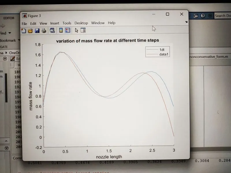
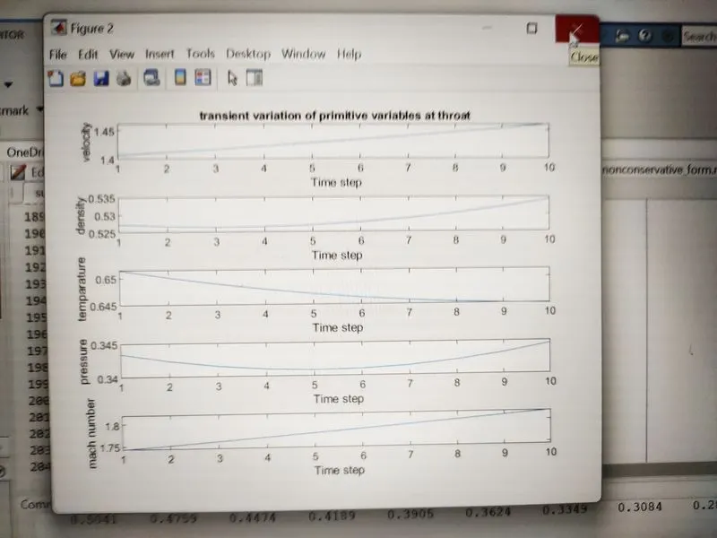
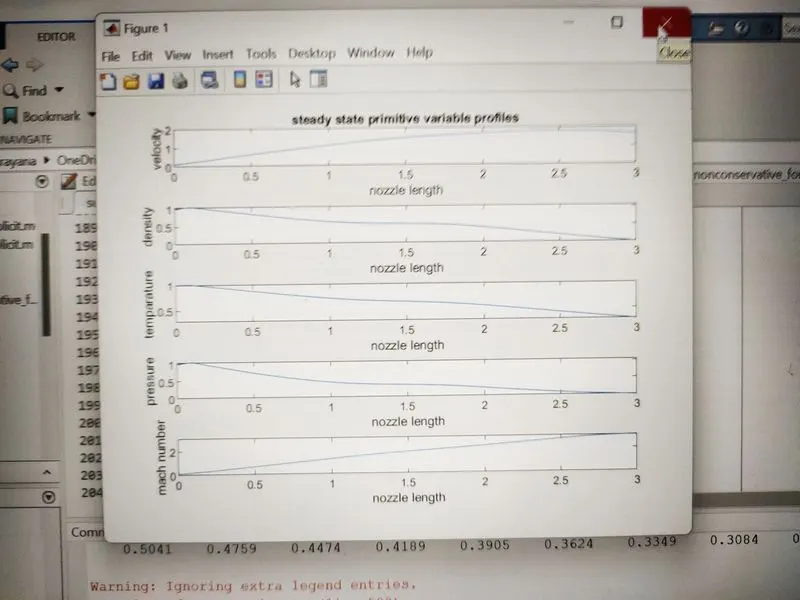
Here are the images of the different plots which were asked in the challenge 1] nozzlelength vs mass flow rate, 2] timestep vs all the primitive variables 3] nozzlelength vs all the primitive variables by observing the graph we can see how the solution is attaing steady state in 2 graph also in 1st nozzle length and mass flow rate vary uncertainly,also in 3rd we see when 'x' increases all the primitive variables slowly becomes steady
2. conservative form (programme)
In this programme, are all same we provide all inputs variables , calculate initial profiles as mentioned above then we calculate using u1,u2,u3, and f1,f2,f3 and create outer time loop and provide the conditions and also do the same steps as we did in non-conservative form programme predictor and corrector step by updating solutions and then apply all the boundary conditions and plot all the neccessary plots as we did before.
clear all
close all
clc

% Inputs
n = 31
x = linspace(0,3,n);
dx = x(2)-x(3);
gamma = 1.4;

% Calculate initial profiles

rho = 1-0.3146*x;
t = 1-0.2314*x; % t = temparature
v = (0.1+1.09*x).*t.^0.5;

for i = 1:n

    if x(i) <= 0.5
    rho(i) = 1;
    t(i) = 1;
    end

    if x(i)> 0.5 && x(i)<= 1.5
    rho(i) = 1 - 0.366*(x(i) - 0.5);
    t(i)  = 1 - 0.167*(x(i) - 0.5);
    end

    if x(i)> 1.5
    rho(i) = 0.634 - 0.3879*(x(i) - 0.5);
    t(i)  = 0.833 - 0.3507*(x(i) - 0.5);
    end

end

% Time steps
nt = 10;
dt = 0.02;

th = round(n/2);

% area
a = 1+2.2*(x-1.5).^2;

v = 0.59./(rho.*a);

u1 = rho.*a;
u2 = rho.*a.*v;
u3 = u1.*(t/(gamma - 1) + (gamma/2)*v.^2);

cfl = (max(v+sqrt(t))*dt/dx);

% Outer time loop
for k = 1:nt

u1_old = u1;
u2_old = u2;
u3_old = u3;

F1 = u2;
F2 = u2.^2./u1 + ((gamma-1)/gamma)*(u3 - (gamma/2)*(u2.^2./u1));
F3 = gamma*u2.*u3./u1 - 0.5*gamma*(gamma-1)*(u2.^3./u1.^2);


   % Predictor method

    for j = 2:n-1

         % continuity equation
         du1dt_p(j) = -(F1(j+1) - F1(j))/dx;

         J2 = (1/gamma)*rho(j)+t(j)*(a(j+1) -a(j))/dx;

         % momemtum equation
         du2dt_p(j) = -(F2(j+1) - F2(j))/dx + J2

        % energy equation
        du3dt_p(j) =  -(F3(j+1) - F3(j))/dx;


       % solution update
       u1(j) = u1(j) + du1dt_p(j)*dt;
       u2(j) = u2(j) + du2dt_p(j)*dt;
       u3(j) = u3(j) + du3dt_p(j)*dt;


    end

    % Predictor update
    rho = u1./a;
    t = (gamma-1)*(u3./u1 - (gamma/2)*(u2./u1).^2);

F1 = u2;
F2 = u2.^2./u1 + ((gamma-1)/gamma)*(u3 - (gamma/2)*(u2.^2./u1));
F3 = gamma*u2.*u3./u1 - 0.5*gamma*(gamma-1)*(u2.^3./u1.^2);

    % Corrector method

for j = 2:n-1
      % continuity equation
         du1dt_c(j) = -(F1(j) - F1(j-1))/dx;

         J2 = (1/gamma)*rho(j)+t(j)*(a(j) -a(j-1))/dx;

         % momemtum equation
         du2dt_c(j) = -(F2(j) - F2(j-1))/dx + J2

        % energy equation
        du3dt_c(j) =  -(F3(j) - F3(j-1))/dx;


end

% Compute the average time derivative

du1dt = 0.5*(du1dt_p + du1dt_c);
du2dt = 0.5*(du2dt_p + du2dt_c);
du3dt = 0.5*(du3dt_p +du3dt_c);


% Final solution update
  for i = 2:n-1
    u1(i) = u1_old(i) + du1dt(i)*dt;
    u2(i) = u2_old(i)+ du2dt(i)*dt;
    u3(i) = u3_old(i) + du3dt(i)*dt;
  end


    % Final update
    rho = u1./a;
    t = (gamma-1)*(u3./u1 - (gamma/2)*(u2./u1).^2);
    v = u2./u2;


  % Apply the boundary conditions
  % Inlet
  u1(1) = a(1);
  u2(1) = 2*u2(2) - u2(3);
  u3(1) = u1(1)*(t(1)/(gamma-1) + 0.5*gamma*v(1)^2);

  % Outlet
  u1(n) = 2*u1(n-1) - u1(n-2);
  u2(n) = 2*u2(n-1) - u2(n-2);
  u3(n) = 2*u3(n-1) - u3(n-2);

  % Pressure
  p = rho.*t;
  % Machnumber
  M = v./sqrt(t);
  % Mass flow rate
  m = rho.*a.*v;

  figure(3)
  hold on
  if k == 1
      plot(x,m);
  end
  if k == 50
      plot(x,m);
  end
  if k == 250
      plot(x,m);
  end
  if k == 500
      plot(x,m);
  end
  if k == 750
      plot(x,m);
  end
  if k == 1200
      plot(x,m);
  end

  rho_throat(k) = rho(th);
  v_throat(k) = v(th);
  t_throat(k) = t(th);
  p_throat(k) = p(th);
  M_throat(k) = M(th);

end
xlabel('nozzle length')
ylabel('mass flow rate')
legend('1dt','50dt','250dt','500dt','750dt','1200dt')
title('variation of mass flow rate at different time steps')


figure(1)
subplot(5,1,1)
plot(x,v)
xlabel('nozzle length')
ylabel('velocity')
title ('steady state primitive variable profiles')
subplot(5,1,2)
plot(x,rho)
xlabel('nozzle length')
ylabel('density')
subplot(5,1,3)
plot(x,t)
xlabel('nozzle length')
ylabel('temparature')
subplot(5,1,4)
plot(x,p)
xlabel('nozzle length')
ylabel('pressure')
subplot(5,1,5)
plot(x,M)
xlabel('nozzle length')
ylabel('mach number')

figure(2)
subplot(5,1,1)
plot(v_throat)
xlabel('Time step')
ylabel('velocity')
title ('transient variation of primitive variables at throat')
subplot(5,1,2)
plot(rho_throat)
xlabel('Time step')
ylabel('density')
subplot(5,1,3)
plot(t_throat)
xlabel('Time step')
ylabel('temparature')
subplot(5,1,4)
plot(p_throat)
xlabel('Time step')
ylabel('pressure')
subplot(5,1,5)
plot(M_throat)
xlabel('Time step')
ylabel('mach number')


figure(3)
plot(x,m);
xlabel('nozzle length')
ylabel('mass flow rate')
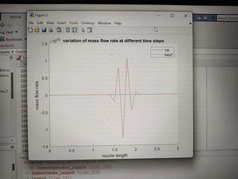
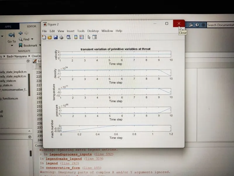
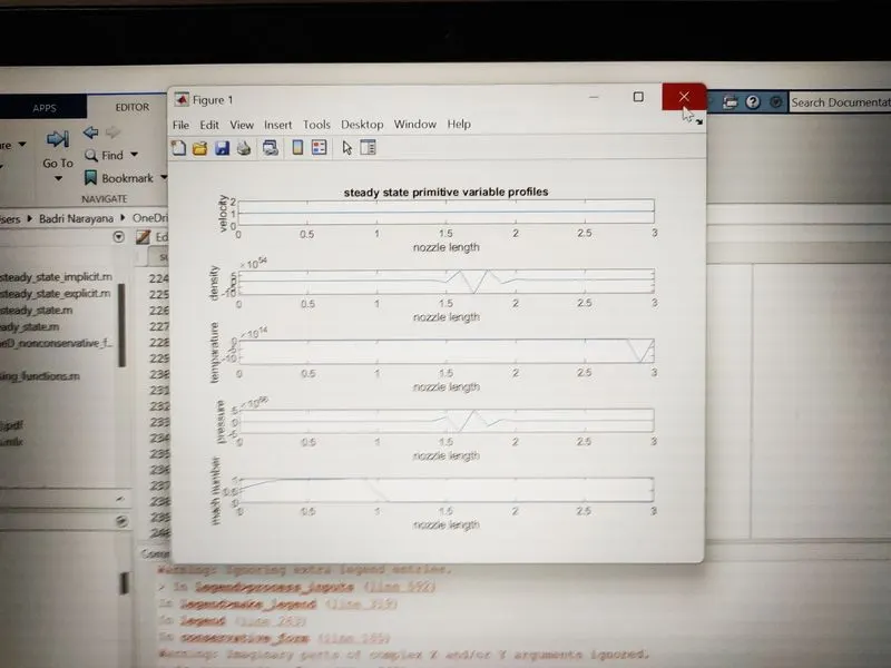
Here are all the neccessary plots for conservative form
1] nozzle length vs mass flow rate 2] time steps vs all the variables 3] nozzle length vs all the variables