Week 9 - FVM Literature Review

AIM:- To describe Finite volume method(FVM).Its interpolation schemes and flux limiters .

SOLUTION THEORY

FINITE VOLUME METHOD

The finite volume method is a method for representing and evaluating parrtial differential equations in the form of algebric equations. In the finite volume method, Volume intergrals in a partial differential equations that contain a divergence term are converted to surface integrals,using divergence theorm. These terms are then evaluated as fluxes at the surface of each finite volume. As the flux entering a given volume is identical to the leaving the adjacent volume,these methods are conservative.
Another advantage of finite volume method is that it is easily formulated to allow for unstructured meshes.The method used in many computational fluid dynamics pakages. "Finite Volume" refers to small volume surrounding each node point on a mesh.

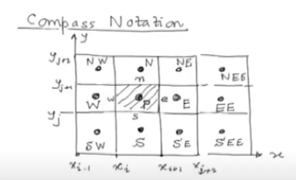
let's consider thr control volume P as and the centroid at the P shown above figure. The above figure hasa set of control volume with centroid located at P. E(East),W(West),N(North),S(South), and furthur point with representation the faces centre is denoted as n,e,s & w. Taking example from heat conduction equation consider small volume 'dv' in control volume P,the integral form of the equation for the small volume is given by,

`int[del/(delx)(alpha*(delT)/(delx))+S]dV=0`

`intdel/(delx)(alpha*(delT)/(delx))dV+intSdV=0`
Now,`dV=A.dx`

`int_w^edel/(delx)(alpha*(delT)/(delx))Adx+intSdV=0`

On solving eqn.

`alpha_eA(delT)/(delx_e)-alpha_wA(delT)/(delx_w)+S_(avg)dv=0`

`S_(avg),alpha` are function of temperature we need to linearize it.

assumin `alpha` is constant

`alphaA((T_E-T_P)/(Deltax))-alphaA((T_P-T_W)/(Deltax))+S_u+S_pT_p=0`

Heat flux out - Heat flux in + source term =0

To calculate Temperature at west and east faces we interpolate values at Tp Te & Tw then using them we can find diffuisvity of the faces. There are differnt types of interpolation those are

1. Upwind interpolation scheme(UDS)

In theis schem we use node in the upwind or upstream of given node generaly used for convection dominated problems.

`f_e = {(f_p,if,(v.n)_e,>,0),(f_E,if,(v.n)_e,<,0):}`

For `v>0 ; u_(i-1/2)≈u_(i-1);u_(i+1/2)≈u_i`

`I_c ≈v(u_i-u_(i-1))/(Δx)`(Backward differencing scheme)

`I_c ≈ v(u_(i+1)-u_i)/(Δx)`(Forward fifferencing scheme)

These approximations satisfy boundedness and is first order accurate in space.

2. Central differencing approximations(CDS)

Approximate values of variable at control volume face centre by linear interpolation of values at two nearest computational nodes.

`f_e =f_Eλ_e + f_p(1-λ_e)` where `λ_e = (x_e-x_p)/(x_E-x_P)`

The linear interpolation is equivalent to that of using central differnce formula for first order derivative and hence this scheme is also determined as central differncing

3. Interpolation Polynomial

`p1(x) = u_L.(x_R-x)/(x_r+x) + u_R.(x-x_L)/(x_R-x_L)`

The interface values are given by

`u_(i-1/2)≈(u_(i-1)+u_i)/2` and `u_(i+1/2) ≈ (u_i+u_(i+1))/2`

`I_c ≈v.(u_(i+1)-u_(i-1))/(2Δx)`

Taylor series approximation polynomial

`u_(i+1/2) = (u_i+u_(i+1))/2 - ((Δx)^2/8).((del^2(u))/(del(x)^2))_(i+1/2) + ...`

The approximation is second order precise .it is the simplest and most widely used interpolation technique for evaluation of gradients required to mesure diffusive fluxes.

FLUX LIMITERS

It is used in numerical schemes to solve problems of fluid dynamics,descriebed by highly coupled non-linear Partial differential equations. If we tend to use low order numerical schemes for solving of governing equations then we might get a high oscillating and unstable solution near disconitinuity if present .Whereas if we tend to use higher order numerical schemes to capture phenomenon more accurately we tend to exploit the computational power unnecessarily. The main idea behind use of flux limiter is to limit the spatial derivative terms near the discontinuities to physical real values so as to maintain physical consistency There are several flux limiter functions.

It is imperative to note that flux limiters are also reffered as slope limiters because they both have same mathametical form and both have effect of limiting solution gradient near shock or discontinuities.

`F(u_(i+1/2)) = f^(low)(i+1/2) - ϕ(r_i)(f^(low)(i+1/2)-f^(high)(i+1/2))`

`F(u_(i-1/2)) = f^(low)(i-1/2)- ϕ(r_i-1)(f^(low)(i-1/2)-f^(high)(i-1/2))`

Here f_low = Low precision flux

f_high = high precision flux

`phi`= flux limiter function `r = (u_i-u_(i-1))/(u_(i+1)-u_i)`