Week 4.1 - Genetic Algorithm
AIM:- (1) Write code for stalagmite function global maxima in matlab.
(2) Explain Ga and code related to it.
(3) Plot for all 3 studies and for Fmaximum and no. for iterations.
Introduction to Optimization
Optimization is the process of making something better. It refers to finding the value of inputs in such a way that we get the best output values,but in mathametical terms , it refers to maximizing or minimizing one or more objective functions , by varying the input parameters.The aim of optimizing is to find hat point or set of points in the search space.
Genetic algorithm
It is method for solving both constrained and unconstrained optimization problems that is based on natural selection, the process that drives biological evolution. The genetic algorithm repeadetly modifies a population of indivsuals solutions. At each steps, the genetic algorithm selects indivisuals from cureent population to be parents and uses them to produce the children for the next generations. Over succesive generations, the population "evolves" toward an optimal solution. You can apply the genetic algorithm to solve variety of optimization problems that are not well suited for optimization algorithms , including problems in which the objective functions is discontinous, non-differntiable or highly nonlinear. The genetic algorithm can address problems of mixed integer programming, where some components are restricted to be integer valued.
The flowchart main steps are as follows:-

The genetic algorithm uses three main types of rules at each step to create next generations:
(1) Selection rules selected the indivisuals , called parents that contribute to the population at the next generations. The selection is generaly stochastic, and can depend on the indivisuals scores.
(2) Crossover rules combine two parents to form children for the next generation.
(3) Mutation rules apply random changes to indivisuals parents to form children.
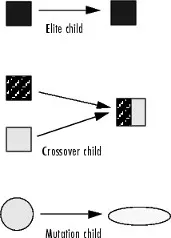
The format for writing GA in MATLAB
X= ga(fun,nvars,a,b,aeq,beq,lb,ub,nonlcon,options)
1. X is the local minima point.
2. fun is the function to be called( in this case the stalagmite_func)
3.nvars indicates no. of variables.
4. 'a' & 'b' are coefficients used to indicate any kind eqaulity exist in function.
5. 'aeq' & 'beq' denotes inequality.
6. 'lb' & 'ub' indicates lower bound and upper bound.
7. 'nonlcon' gives two vector representing inequalities and equalities.
8. 'options' is used to perform additional operations like increasing and decreasing population size with help of "optimoptions".
PROCEDURE:
(1) The stalagmite functions is defined seperately. This function is later called in to the GA program.
(2) Now we define the x & y inputs using linspace command.
(3) Then the input vectors are transformed into array [xx yy], so that it can be used to evaluate functions of two variables and plot 3-D mesh/surface plots.
(4) Now the values in the different matrix created can be put as an input into the function that we created by calling it and can get values for x & y.
(5) SInce we got value of functions at various values, we now need to calculate the maxima value using "ga" command which is inbulit in MATLAB But matlab inbulit only finds global minima to find maximum we use negative sign so we get inverse which is maxima .
(6) Then total no. of times "ga" needs to run to be defined using "num_ cases" and with help of "for" loop ga is made to run for each iteration and value is stored in an array.
(7)The total time is calculated using the 'tic' and 'toc' command at the start and end of "for" loop respectively.
(8) The results are then plotted using the surfc command and plot command .
(9) GA is made to run for 3 iterations, with each iteration having bounded inputs , unbounded inputs, and incresed size population bounded size.
The equation for stalagmite_func is as follows:
f1x= (sin(5.1*pi*x+.5))^6
f1y= (sin(5.1*pi*y+.5))^6
f2x= (exp(-4*log(2)*(x-0.0667)^2/.64)
f2y= (exp(-4*log(2)*(y-0.0667)^2/.64)
f= -(f1x*f1y*f2y*f2x) ( negative sign is used to inverse and find maxima value)
function [ F ] = stalagmite_func(input_vector)

x = input_vector(1);
y = input_vector(2);

f1 = (sin(5.1*pi*x +0.5))^6;

f2 = (sin(5.1*pi*y +0.5))^6;

f3 = exp(-4*log(2)*((x-0.0667)^2)/(0.64));

f4 = exp(-4*log(2)*((y-0.0667)^2)/(0.64));

F= -f1*f2*f3*f4;

end
1ST Iterration:
Unbounded searchspace means no defined bounds.
clear all
close all
clc

% Defining our search space
x= linspace(0,0.9,150);
y= linspace(0,0.9,150);

 % Ga run for 50 iterations
num_cases=100
% creating 2-d meshgrid

[xx yy]= meshgrid(x,y);

%stlagmite function

for i=1:length(xx)
    for j=1:length(yy)

        input_vector(1) = xx(i,j);
        input_vector(2) = yy(i,j);

        f(i,j)= stalagmite_func(input_vector);
    end
end


% count time
tic

for i= 1:num_cases
    [inputs  f_opt(i)] = ga(@stalagmite_func,2);
    x_opt= inputs(1);
    y_opt= inputs(2);
% ga gives us minima we inverse it to find maxima
    opt_f = -(f_opt);
end

% study time clock end
study_time1= toc

% generation of stalgmite function
figure(1)
subplot(2,1,1)
hold on
surfc(xx,yy,f)
xlabel('x value')
ylabel('y value')
% to bring smoothnes without shading lines
shading interp
hold on
%plotting with 3d
plot3(x_opt,y_opt,f_opt,'marker','o','markersize',5,'markerfacecolor','r')

title('Unbound Inputs')
subplot(2,1,2)

plot(opt_f)
xlabel('No. of iterations')
ylabel('Function max')
RESULTS
Study _time= 4.64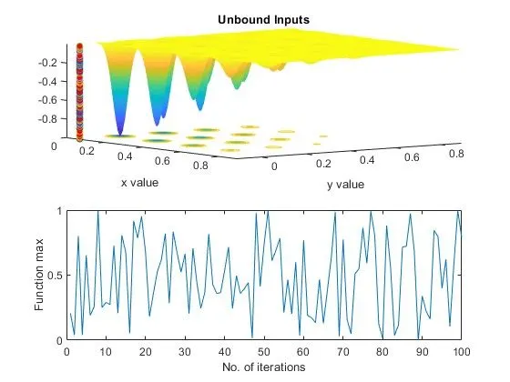
2nd Iteration
here upper and lower bounds are defined in otherwords we define space within which global maxima is to be found.
clear all
close all
clc

% Defining our search space
x= linspace(0,0.9,150);
y= linspace(0,0.9,150);

 % Ga run for 50 iterations
num_cases=100
% creating 2-d meshgrid

[xx yy]= meshgrid(x,y);

%stlagmite function

for i=1:length(xx)
    for j=1:length(yy)

        input_vector(1) = xx(i,j);
        input_vector(2) = yy(i,j);

        f(i,j)= stalagmite_func(input_vector);
    end
end

%bounded limits
% count time
tic

for i= 1:num_cases
     % Function is stalagmite_func & variables 2
    % eq & aeq= [] [] [][] ( as its null here)
    % lower bound an upper bound is[o;o],[1;1]
    [inputs  f_opt(i)] = ga(@stalagmite_func,2,[],[],[],[],[0;0],[.9;.9]);
    x_opt= inputs(1);
    y_opt= inputs(2);
% ga gives us minima we inverse it to find maxima
    opt_f = -(f_opt);
end

% study time clock end
study_time2= toc

% generation of stalgmite function
figure(2)
subplot(2,1,1)
hold on
surfc(xx,yy,f)
xlabel('x value')
ylabel('y value')
% to bring smoothnes without shading lines
shading interp
hold on
%plotting with 3d
plot3(x_opt,y_opt,f_opt,'marker','o','markersize',5,'markerfacecolor','r')

title('Bounded Inputs')
subplot(2,1,2)

plot(opt_f)
xlabel('No. of iterations')
ylabel('Function max')
RESULTS
Study_time=6.56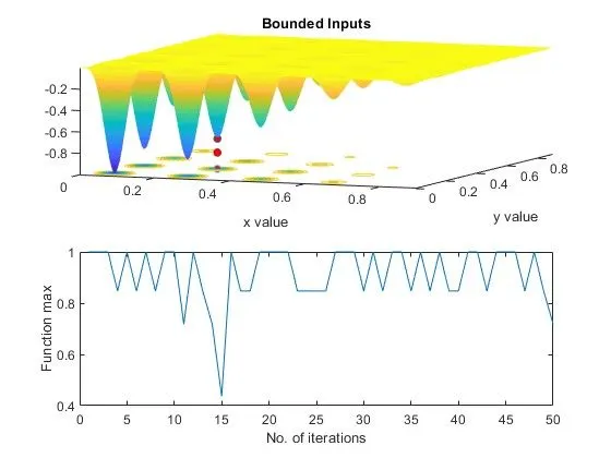
3rd Iterration
In this case population size is increased as to converge global maxima
clear all
close all
clc

% Defining our search space
x= linspace(0,0.9,150);
y= linspace(0,0.9,150);

 % Ga run for 50 iterations
num_cases=150
% creating 2-d meshgrid

[xx yy]= meshgrid(x,y);

%stlagmite function

for i=1:length(xx)
    for j=1:length(yy)

        input_vector(1) = xx(i,j);
        input_vector(2) = yy(i,j);

        f(i,j)= stalagmite_func(input_vector);
    end
end

% 3rd iterartion increasing population isze

options= optimoptions('ga');
options= optimoptions(options,'Populationsize', 470);


for i= 1:num_cases
    [inputs  f_opt(i)] = ga(@stalagmite_func,2,[],[],[],[],[0;0],[.9;.9],[],[],options);
    x_opt= inputs(1);
    y_opt= inputs(2);
% ga gives us minima we inverse it to find maxima
    opt_f = -(f_opt);
end

% study time clock end
study_time3= toc

% generation of stalgmite function
figure(3)
subplot(2,1,1)
hold on
surfc(xx,yy,f)
xlabel('x value')
ylabel('y value')
% to bring smoothnes without shading lines
shading interp
%plotting with 3d
plot3(x_opt,y_opt,f_opt,'marker','o','markersize',5,'markerfacecolor','r')

title('Bound inputs with increase population size')
subplot(2,1,2)

plot(opt_f)
xlabel('No. of iterations')
RESULTS
Study time=222.74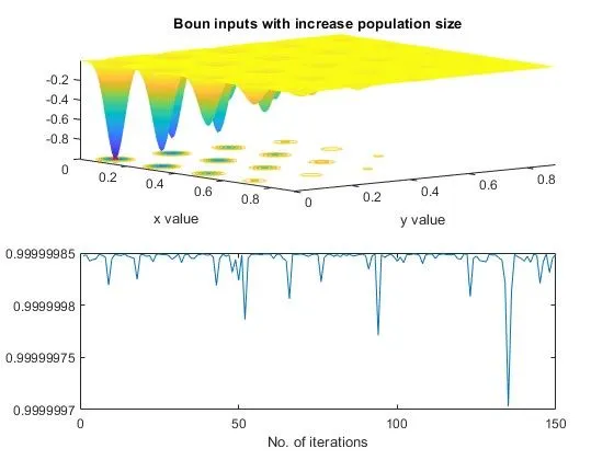
ERROR: incase of options here i wrote option.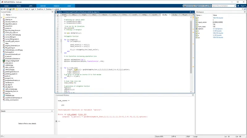
REFERENCE
https://in.mathwhttps://in.mathworks.com/help/gads/ga.htmlorks.com/help/gads/ga.html