Week 9 - FVM Literature Review

AIM:

The objective of the report is to discuss major differences between finite difference method and finite volume method and the need for interpolation schemes and flux limiters in FVM.

LITERATURE REVIEW:

FINITE DIFFERENCE METHOD -

• In FDM, the differential form of governing equation is solved.
• The domain is discretized into a set of grid points and solution of flux variables are calculated at the grid points.
• The governing equations are valid only at the grid points.

FINITE VOLUME METHOD -

• In FVM, the integral form of governing equation is solved.
• The domain is discretized into a set of control volumes and solution of flux variables are calculated at grid point present inside the control volume. In maximum cases, centroid is taken as the grid point.
• The governing equations are valid in the entire volume.
• The advantage of FVM over FDM is, for complex geometries and moving parts, the FDM is difficult to solve as grid lines are not aligned along x,y,z axis. So FVM gives accurate results.

Example -

Consider Steadt state 1D linear heat conduction equation

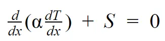, where α - thermal diffusivity, S - Source term responsible for heat generation

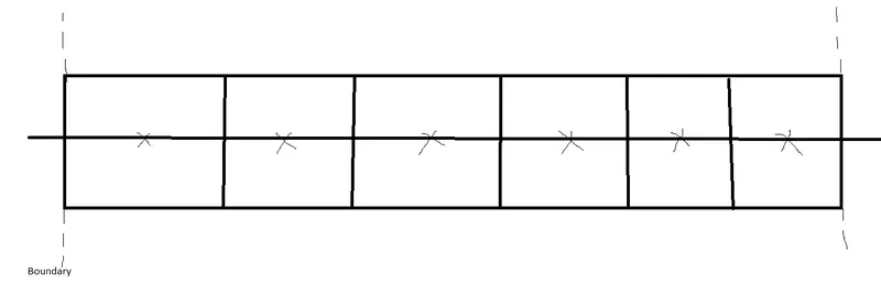
Now, discretize the domain into a set of finite control volume

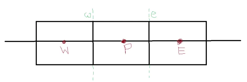
Nomenclature for FVM -

P is the centroid of the working cell to which governing equations are applied.

E is the centroid of control volume present to the right side of P

W is the centroid of control volume present to the left side of P

e is the right face of control volume of centroid P

w is the left face of control volume of centroid P

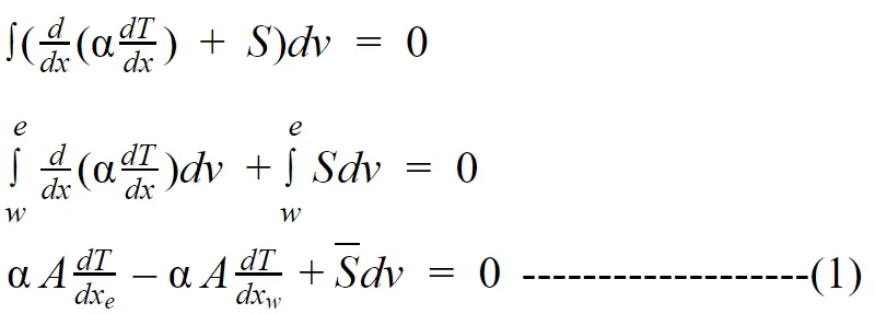
Applying governing equation to control volume P, we get

NEED OF INTERPOLATION -

To solve eq(1), we need to calculate the temperature gradient at the faces of control volume. In FVM, the field variables are calculated at the centroid of the control volume. So, the field variables at faces are calculated by interpolation.

Interpolation Schemes :

Let, ϕ is the field variable. Temperature, velocity, pressure, density all are field variables. In the eq(1), Temperature is the field variable.

Fe is the flow of information at face 'e'. Fe > 0 means information flows in the direction of area vector

Fe < 0 means information flows in the opposite direction to area vector

1) Linear/Central differencing scheme -

ϕe = 0.5*(ϕP + ϕE)

Where ϕe - Field variable value at the face e

ϕP - Field variable value at P

ϕE - Field variable value at E

2) Upwind differencing scheme -

The upward differencing scheme is first-order accurate. It is stable but have large numerical diffusion effect. It is used to find initial solution as it gives stable result.

ϕe = ϕP , when Fe > 0

= ϕE , when Fe < 0

3) Linear Upwind differencing scheme -

The Linear upward differencing scheme is second-order accurate. It is more accurate than upwind differencing scheme.

ϕe = ϕP + (∇ϕP)*r , when Fe > 0

= ϕE + (∇ϕE)*r , when Fe < 0

4) Quick scheme -

The Quick scheme is third-order accurate. It uses quadratic term or interpolation. Quick scheme is more accurate but wiggles (or) oscillations will occur.

ϕe = (6ϕP - ϕW + 3ϕE)/8 , when Fe > 0

= (6ϕE - ϕEE + 3ϕP)/8 , when Fe < 0

5) TVD scheme -

TVD scheme is mainly used to solve hyperbolic PDE. The tendency of oscillations in quick scheme is overcome by using TVD scheme.

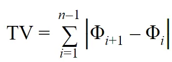
The Total variation diminishing scheme is monotonicity preserving. The total variation must not increase it diminishes with time.

ϕe = ϕP + 0.5*ψ(r)*(ϕE-ϕP), where ψ(r) is flux limiter function

r = (ϕP - ϕW)/(ϕE - ϕP)

FLUX LIMITER -

Flux limiters ψ(r) are used to diminish the overshoots and undershoots to the solution which means no local maximum and minima are created. They are used when sharp wave fronts are present. For smoothly changing waves, the flux limiters do not operate and the spatial derivatives can be represented by higher order approximations without introducing spurious oscillations.

Some flux-limiter functions -

1) Van-Leer function - ψ(r) = (r + |r|)/(1+|r|)

2) Super-bee function - ψ(r) = max[0, min(2r,1), min(r,2)]

So, the main advantage of using flux limiters is the calculated solution variables lies within range of neighbouring cell values. In the above case, ϕP ≤ ϕe ≤ ϕE (or) ϕE ≤ ϕe ≤ ϕP.

From eq 1,

By using backward and forward gradient scheme in eq1, we get

By interpolation schemes,

Te = TP + 0.5*ψ(re)*(TE - TP), where re = (TP - TW)/(TE - TP)

Tw = TW + 0.5*ψ(rw)*(TP - TW), where rw = (TW - TWW)/(TP - TW)

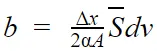
By substituting the above equation in eq(2), we get

,

where aP = 1+0.5*ψ(re)-0.5*ψ(rw)

aE = 0.5*ψ(re)

aW = 1-0.5*ψ(rw)