Week 9 - FVM Literature Review
The Finite Volume Method (FVM)
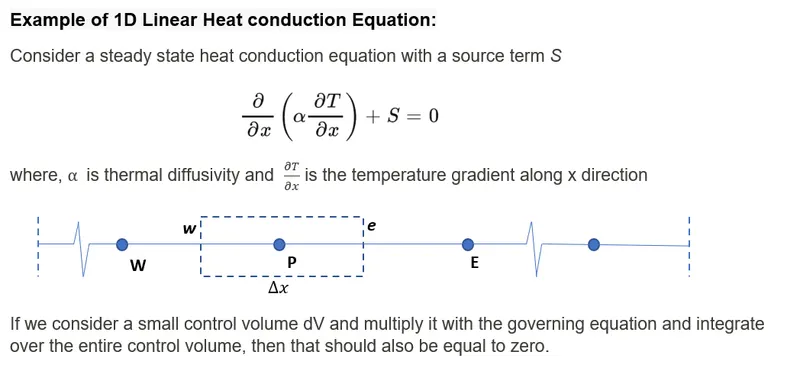
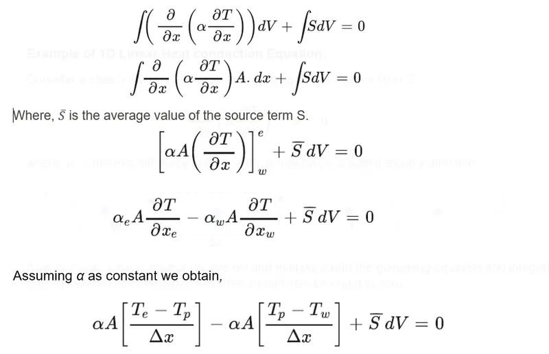
The Finite Volume Method (FVM) is an approach to numerically approximate PDEs in their integral form. FVM can be used on all differential equations, which can be written in the divergence form. Thus, the PDE is written using divergence operators and then integrated over the control volume. The Gauss Divergence theorem can then be used to convert the volume integral into surface integrals. The problem is then reduced from integrating the differential of the dependent variable inside of the control volume (or cell) into surface integrals of the fluxes of the dependent variable across the boundary of the cells. These integrals can usually be calculated using suitable numerical approximation methods.
Differences between FVM and FDM:
The differential form of the PDE to be solved is used in a finite difference method (FDM) discretization. The integral form of the conservation rules, rather than their differential form, is used in FVM.
The computational domain in FDM is typically divided into hexahedral cells (the grid), with the solution obtained at each nodal point. The computational domain is discretized into finite volumes in FVM, and the governing equations are solved for each volume. The conserved variable's fluxes are calculated across the surface of the control volume.
The discretization in FDM produces a set of equations for the variable at nodal points, and after a solution is obtained, the solution is represented discretely. The approximate solution produced by FVM is discrete, however the variables are usually positioned at cell centers rather than nodal points. Sometimes the values are also stored at face centers of the control volume which are obtained using interpolation.
Interpolation schemes
When FVM is used, it is required to employ interpolation schemes to approximate the property values placed at the control volume boundaries (cell faces). The corresponding properties located at the center of the adjacent control volumes are used as the interpolation nodes.
There are different schemes available to compute the value at the surfaces of the control volume like
- Upwind interpolation
- Linear interpolation
- Quadratic upwind differencing scheme: the Quick scheme
- Hybrid, Total variation dimension (TVD) scheme and
- Essentially non-oscillatory (ENO) interpolation scheme etc.
Flux Limiters:
Low-order schemes for convective fluid flow are normally stable but relatively dissipative in nature around points of discontinuity or shocks, whereas higher-order systems are unstable and show oscillations in the region of discontinuity. High resolution systems are those that are highly accurate and free of oscillations.
Flux limiter functions are used to tune higher order and low order schemes so that the final scheme provides higher order accuracy in the smooth area of the flow while maintaining first order accuracy near shocks and discontinuities.