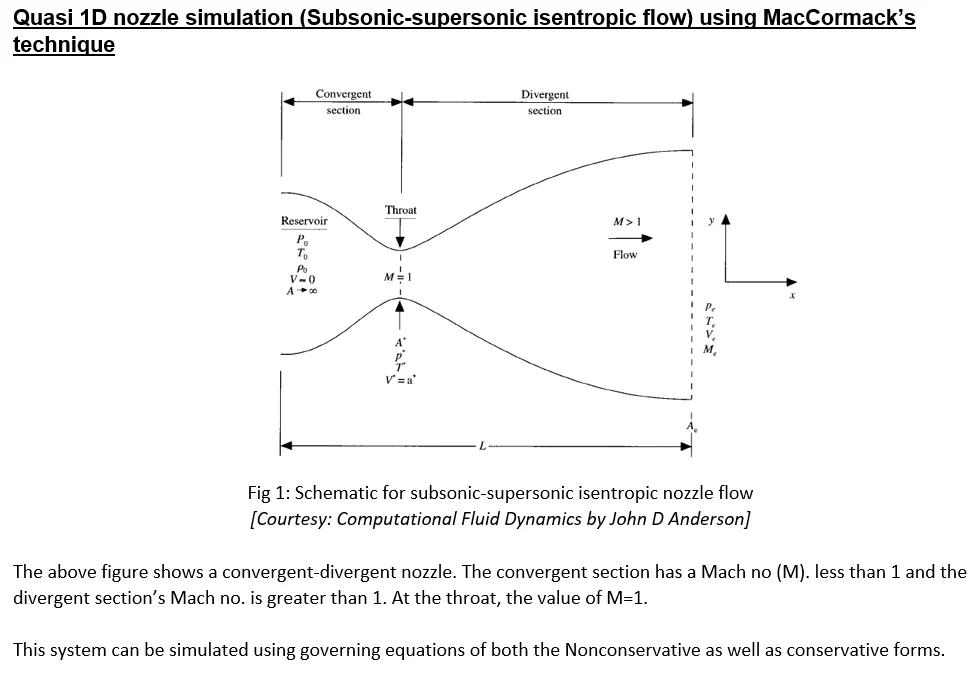
Week 7 - Simulation of a 1D Super-sonic nozzle flow simulation using Macormack Method

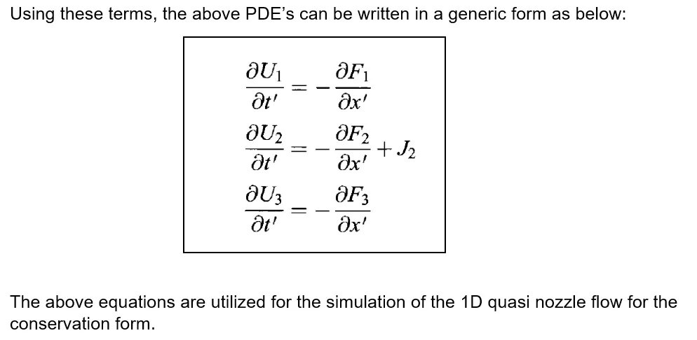
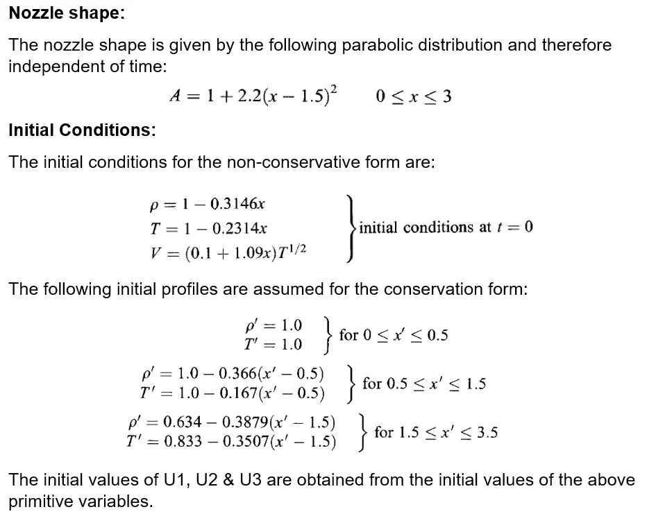
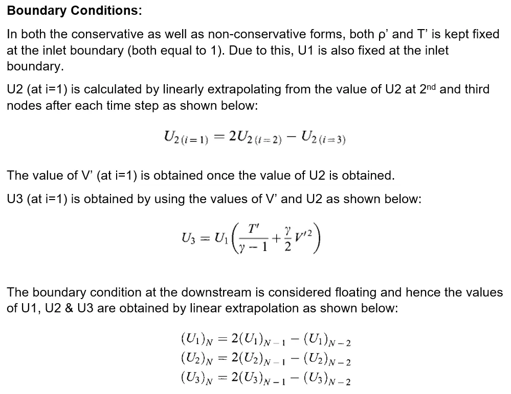
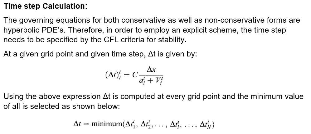
MATLAB Code

MainProgram:

%%%%QUASI 1D NOZZLE SIMULATION USING CONSERVATIVE & NON-CONSERVATIVE APPROACH%%%%%%
%%%%ARGHAJIT CHAKRABORTY%%%%%%%%%%%%%%%%%%%%%%%%%%%%%%%%%%%%%%%%%%%%%%%%%%%
clear all;
close all;
clc;

%%%%%%%%%%%%%%INPUTS%%%%%%%%%%%%%%%%%%%%%%%%%%%%%%%%%%%%%%
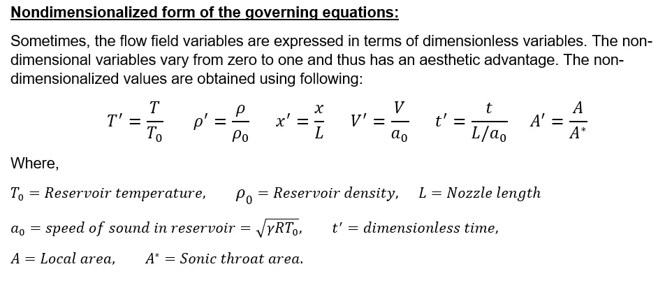
L = 3;
nodes=[61,31];
for i=1:2
n = nodes(i) ;
x = linspace(0,3,n);
nt =1400;
dx = x(2)-x(1);
a = 1+2.2*(x-1.5).^2; % area profile 
c = 0.5 ; % courant number
gamma = 1.4 ; % specific heat ratio 
throat = find(a==1);

%%%%%%%%%%%%SOLUTION#######################################
% Solution for non conservative form of governing equations

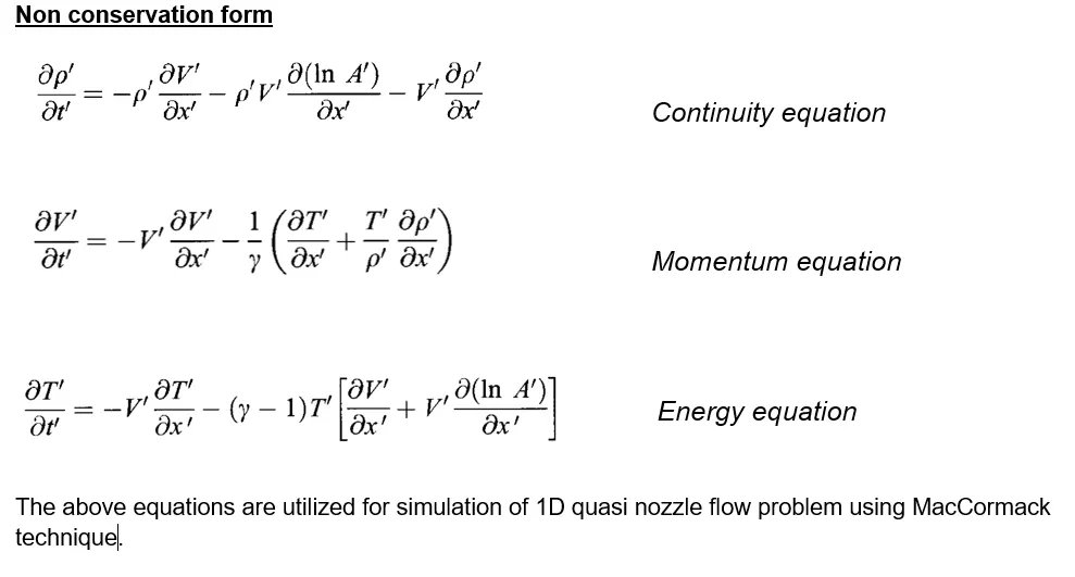
[rho,v,t,p,rho_th,t_th,p_th,m_nc,M,M_th] = non_conservative(x,dx,n,nt,gamma,a,throat,c);

% Solution for conservative form of governing equations
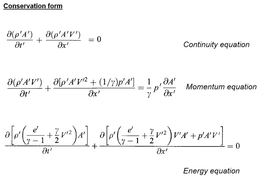
[rho_c,v_c,t_c,p_c,rho_th_c,t_th_c,p_th_c,m_c,M_c,M_th_c] =conservative(x,dx,n,nt,gamma,a,throat,c);

%%%%%%%%%%%%%%PLOTTING%%%%%%%%%%%%%%%%%%%%%%%%%%%%%%%%%%%%%
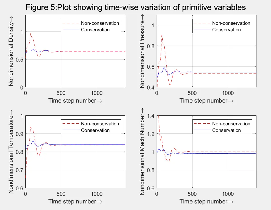
% Plotting Density , pressure, temperature & Mach number wrt time step:
figure(5);
subplot(2,2,1);
plot(rho_th,'r','linestyle','--' );
hold on
plot(rho_th_c,'b');
hold off
grid on
ylabel('Nondimensional Density\rightarrow');
xlabel('Time step number\rightarrow');
legend('Non-conservation','Conservation')
axis([0 1400 0 1.3]);

subplot(2,2,2);
plot(p_th,'r','linestyle','--');
hold on
plot(p_th_c,'b');
hold off
grid on
xlabel('Time step number\rightarrow');
ylabel('Nondimensional Pressure\rightarrow');
legend('Non-conservation','Conservation')
axis([0 1400 0.4 1.1]);

subplot(2,2,3);
plot(t_th,'r','linestyle','--');
hold on
plot(t_th_c,'b');
hold off
grid on
xlabel('Time step number\rightarrow');
ylabel('Nondimensional Temperature\rightarrow');
legend('Non-conservation','Conservation')
axis([0 1400 0.6 1]);

subplot(2,2,4);
plot(M_th,'r','linestyle','--');
hold on
plot(M_th_c,'b');
hold off
grid on
xlabel('Time step number\rightarrow');
ylabel('Nondimensional Mach Number\rightarrow');
legend('Non-conservation','Conservation')
axis([0 1400 0.6 1.4]);
sgtitle ('Figure 5:Plot showing time-wise variation of primitive variables','FontSize',14);

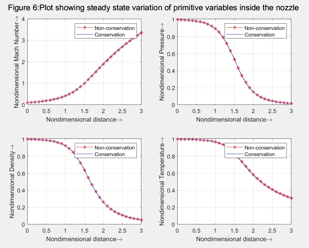
%Plotting variation of P,Rho,T,M wrt nozzle length
figure(6);
subplot(2,2,1);
plot(x,M,'r','marker','*');
hold on
plot(x,M_c,'b');
hold off
grid on
ylabel('Nondimensional Mach Number\rightarrow');
xlabel('Nondimensional distance\rightarrow');
legend('Non-conservation','Conservation')
axis([0 3 0 4]);

subplot(2,2,2);
plot(x,p,'r','marker','*');
hold on
plot(x,p_c,'b');
hold off
grid on
ylabel('Nondimensional Pressure\rightarrow');
xlabel('Nondimensional distance\rightarrow');
legend('Non-conservation','Conservation')
axis([0 3 0 1.01]);

subplot(2,2,3);
plot(x,rho,'r','marker','*');
hold on
plot(x,rho_c,'b');
hold off
grid on
ylabel('Nondimensional Density\rightarrow');
xlabel('Nondimensional distance\rightarrow');
legend('Non-conservation','Conservation')
axis([0 3 0 1.01]);

subplot(2,2,4);
plot(x,t,'r','marker','*');
hold on
plot(x,t_c,'b');
hold off
grid on
ylabel('Nondimensional Temperature\rightarrow');
axis([0 3 0 1.01]);
xlabel('Nondimensional distance\rightarrow');
legend('Non-conservation','Conservation')
sgtitle ('Figure 6:Plot showing steady state variation of primitive variables inside the nozzle','FontSize',14);

% Mass flow rate comparison for both conservative and non consevative forms
figure(7);
plot(x, m_nc, 'b');
hold on;
plot(x, m_c, 'r');

line([0 3], [0.579 0.579]);%Analytical solution
legend('Nonconservative','Conservative','Exact solution','location','best');
leg=legend('show');
title(leg,'Legend');
strx=sprintf('Figure 7:Steady state mass flow variations\nNonconservation vs Conservation\nn=%d',n);
title(strx,'FontSize',12);
xlabel('Nondimensional distance (x/L)\rightarrow');
ylabel('Nondimensional mass flow(\rhoVA/\rho_0a_0A^*)\rightarrow');
hold off
Name = {'Density*','Temperature*','Pressure*','Mach no.*'};
T = table([0.6340;0.8330;0.5280;1.0000],[rho_th(nt);t_th(nt);p_th(nt);M_th(nt)],[rho_th_c(nt);t_th_c(nt);p_th_c(nt);M_th_c(nt)]);
T.Properties.RowNames = Name;
str = sprintf('Nonconservative_%d',n);
str1 = sprintf('Conservative_%d',n);
T.Properties.VariableNames = {'Exactsolution',str,str1}
T(:,1:3);
end

Function for conservation form:

%%QUASI 1D CONSERVATION FORM%%%%%%%
function [rho_c,v_c,t_c,p_c,rho_th_c,t_th_c,p_th_c,m_c,M_c,M_th_c] = conservative(x,dx,n,nt,gamma,a,throat,c)

mcplot = [1,100,200,700];
% Compute initial profile
for i = 1:n
    if  x(i) >= 0 && x(i) < 0.5
    rho_c(i) = 1;
    t_c(i) = 1;
    elseif x(i) >= 0.5 && x(i) < 1.5
    rho_c(i) = 1.0 -0.366*(x(i) - 0.5);
    t_c(i) = 1.0 - 0.167*(x(i) - 0.5);
    elseif x(i) >= 1.5 && x(i) <= 3.0
    rho_c(i) = 0.634 - 0.3879*(x(i) - 1.5);
    t_c(i) = 0.833 - 0.3507*(x(i) - 1.5);
    end
end
% Initial velocity and pressure:
v_c = 0.59./(rho_c.*a);
p_c = rho_c.*t_c;

% Solution vectors:
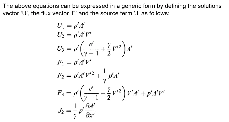
U1 = rho_c.*a;
U2 = rho_c.*a.*v_c;
U3 = rho_c.*a.*((t_c./(gamma - 1)) + (gamma/2)*v_c.^2);

% Outer time Loop
for k = 1:nt

U1_old = U1;
U2_old = U2;
U3_old = U3;

% Adaptive Time-step control:
dt = min(c.*dx./(sqrt(t_c) + v_c));

% Defining the flux vectors:
F1 = U2;
F2 = (U2.^2./U1) + ((gamma-1)/gamma)*(U3 - (gamma*U2.^2)./(2*U1));
F3 = (gamma*U2.*U3./U1) - (gamma*(gamma-1)/2)*(U2.^3./U1.^2);

% MacCormack Technique
for j = 2:n-1
% Defining the source term:
J2(j) = (1/gamma).*rho_c(j).*t_c(j).*((a(j+1)-a(j))/dx);

%Predictor step:

dU1dt_p(j) = -(F1(j+1) - F1(j))/dx;            %continuity eq
dU2dt_p(j) = -((F2(j+1) - F2(j))/dx) + J2(j);  %Momentum equation
dU3dt_p(j) = -(F3(j+1) - F3(j))/dx;            %Energy equation

% Solution update
U1(j) = U1(j) + dU1dt_p(j)*dt;
U2(j) = U2(j) + dU2dt_p(j)*dt;
U3(j) = U3(j) + dU3dt_p(j)*dt;
end

% Updating the primitive variables and flux vectors:
rho_c = U1./a;
v_c = U2./U1;
t_c = (gamma -1)*(U3./U1 - (gamma/2)*v_c.^2);
p_c = rho_c.*t_c;

% Corrector step:
F1 = U2;
F2 = (U2.^2./U1) + ((gamma-1)/gamma)*(U3 - (gamma*U2.^2)./(2*U1));
F3 = (gamma*U2.*U3./U1) - (gamma*(gamma-1)/2)*(U2.^3./U1.^2);
for j = 2:n-1
    
% Updating the source term:
J2(j) = (1/gamma)*rho_c(j).*t_c(j)*((a(j)-a(j-1))/dx);

% Corrector step:
dU1dt_c(j) = -(F1(j) - F1(j-1))/dx;
dU2dt_c(j) = -((F2(j) - F2(j-1))/dx) + J2(j);
dU3dt_c(j) = -(F3(j) - F3(j-1))/dx;
end
% Updating the solution vectors after corrector step:
% Averaging the predictor and corrector steps:
dU1dt = 0.5*(dU1dt_p + dU1dt_c);
dU2dt = 0.5*(dU2dt_p + dU2dt_c);
dU3dt = 0.5*(dU3dt_p + dU3dt_c);
% Calculating the new solution vectors:
for j = 2:n-1
U1(j) = U1_old(j) + dU1dt(j)*dt;
U2(j) = U2_old(j) + dU2dt(j)*dt;
U3(j) = U3_old(j) + dU3dt(j)*dt;
end
% Applying BC:
% Inlet conditions
v_c(1)=2*v_c(2)-v_c(3);
U1(1)=a(1);
U2(1) = 2*U2(2) - U2(3);
U3(1)=U1(1)*(1/(gamma-1)+(0.5*gamma*v_c(1)^2));
% Outlet conditions:
U1(n) = 2*U1(n-1) - U1(n-2);
U2(n) = 2*U2(n-1) - U2(n-2);
U3(n) = 2*U3(n-1) - U3(n-2);
% Final updation of the primitive variables:
rho_c = U1./a;
v_c = U2./U1;
t_c = (gamma -1)*(U3./U1 - (gamma/2)*v_c.^2);
p_c = rho_c.*t_c;

% Mach Number and mass flow rate:
M_c = v_c./sqrt(t_c);
m_c = rho_c.*a.*v_c;

% Calculating values of specific quantites at the throat:
M_th_c(k) = M_c(throat);        % Mach Number
p_th_c(k) = p_c(throat);        % Pressure Ratio
t_th_c(k) = t_c(throat);        % Non-dimensional Temperature
rho_th_c(k) = rho_c(throat);    % Density Ratio

% Comparison of non-dimensional mass-flow rates at different times:

  for j=1:1:4
        if k == mcplot(j)
            for s=1:1:n 
              mc_call(s,j) = m_c(s);                            % Store the values of 'm_c' corresponding to the 'k'
            end                                                 % values in the 'mcplot' matrix for plotting purpose
         end
  end

end
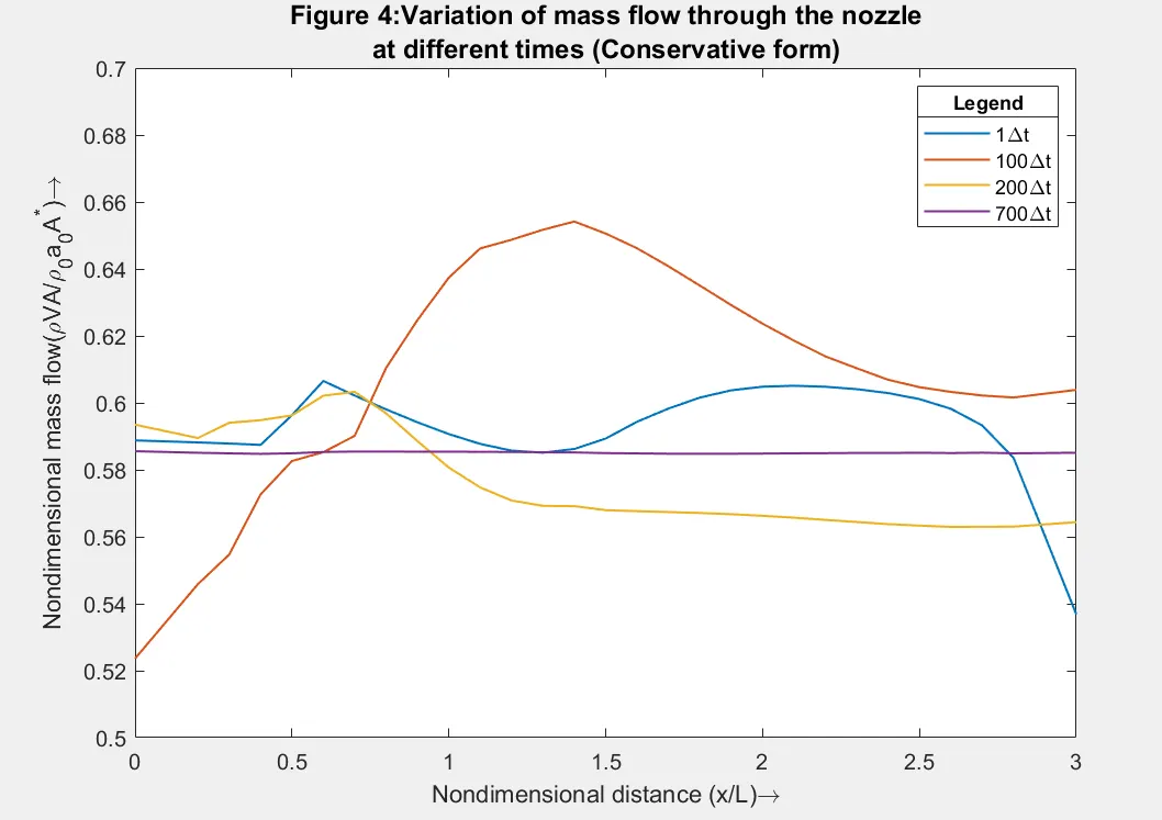
    figure(4);
    plot(x,mc_call,'linewidth',1.0);
    axis([0 3 0.5 0.7]);
    legendcell = strcat(string(mcplot(1:4)),"\Deltat" );
    legend(legendcell,'location','northeast');
    leg=legend('show');
    title(leg,'Legend');
    title({'Figure 4:Variation of mass flow through the nozzle'; 'at different times (Conservative form)'},'FontSize',12);
    xlabel('Nondimensional distance (x/L)\rightarrow');
    ylabel('Nondimensional mass flow(\rhoVA/\rho_0a_0A^*)\rightarrow');

end

Function for non-conservation form:

%%QUASI 1D NON-CONSERVATION FORM%%%%%%%
function [rho,v,t,p,rho_th,t_th,p_th,m_nc,M,M_th] = non_conservative(x,dx,n,nt,gamma,a,throat,c)
mncplot = [1,50,100,150,200,700];
% Using MacCormack's method to solve non- conservative form of 1-D supersonic nozzle equation.
rho = 1- 0.3146*x;
t = 1 - 0.2314*x;
v = (0.1+1.09*x).*t.^0.5;
% Outer time loop
for k = 1:nt
rho_old =rho;
t_old =t;
v_old =v;
%Adaptive time-step control
dt = min(c.*dx./(sqrt(t)+v));
% predictor method
for j=2:n-1
dvdx =( v(j+1)-v(j))/dx;
drhodx =( rho(j+1)-rho(j))/dx;
dtdx =( t(j+1)-t(j))/dx;
dlogadx = (log(a(j+1))-log(a(j)))/dx;
% continuity equation
drhodt_p(j) = - rho(j)*dvdx - rho(j)*v(j)*dlogadx -v(j)*drhodx;
% Momentum equation
dvdt_p(j) = - v(j)*dvdx - (1/gamma )*(dtdx +(t(j)/rho(j))*drhodx);
% Energy equation
dtdt_p(j) = -v(j)*dtdx - (gamma-1)*t(j) *(dvdx +v(j)*dlogadx);
% solution update
rho(j) = rho(j) + drhodt_p(j)*dt;
v(j) = v(j) + dvdt_p(j)*dt;
t(j) = t(j) + dtdt_p(j)*dt;
end
% corrector method
for j = 2:n-1
dvdx =( v(j)-v(j-1))/dx;
drhodx =( rho(j)-rho(j-1))/dx;
dtdx =( t(j)-t(j-1))/dx;
dlogadx = (log(a(j))-log(a(j-1)))/dx;
% Continuity Equation
drhodt_c(j) = - rho(j)*dvdx - rho(j)*v(j)*dlogadx -v(j)*drhodx;
% Momentum Equation
dvdt_c(j) = - v(j)*dvdx - (1/gamma )*(dtdx +(t(j)/rho(j))*drhodx);
% Energy Equation
dtdt_c(j) = -v(j)*dtdx - (gamma-1)*t(j) *(dvdx +v(j)*dlogadx);
end
% compute average time derivative
drhodt = 0.5*(drhodt_p+drhodt_c);
dvdt = 0.5*(dvdt_p+dvdt_c);
dtdt = 0.5*(dtdt_p+dtdt_c);
% Final solution update
for i = 2:n-1 
rho(i) = rho_old(i)+drhodt(i)*dt;
v(i) = v_old(i)+dvdt(i)*dt;
t(i) =t_old(i)+dtdt(i)*dt;
end
% BC
% Inlet Boudary conditions
v(1) = 2*v(2) -v(3);
rho(1) = 1;
t(1) = 1;
% Outlet Boudary conditions
v(n) = 2*v(n-1)-v(n-2);
rho(n) = 2*rho(n-1)-rho(n-2);
t(n) = 2*t(n-1)-t(n-2);
% Defining the values for pressure, mass flow rate and mach number:
p = rho.*t; %Non-Dimensional Pressure
m_nc = rho.*a.*v; %Non-Dimensional Mass flow rate
M = v./sqrt(t); %Mach Number
%Calculation of Quantities at the Throat point of the nozzle:
t_th(k) = t(throat);
p_th(k) = p(throat);
rho_th(k) = rho(throat);
M_th(k) = M(throat);
% Comparison of non dimensional mass flow rates at different times:

  for j=1:1:6
        if k == mncplot(j)
            for s=1:1:n 
              mnc_call(s,j) = m_nc(s);                               % Store the values of 'm_nc' corresponding to the 'mnc_plot'
            end                                                 
         end
  end

end
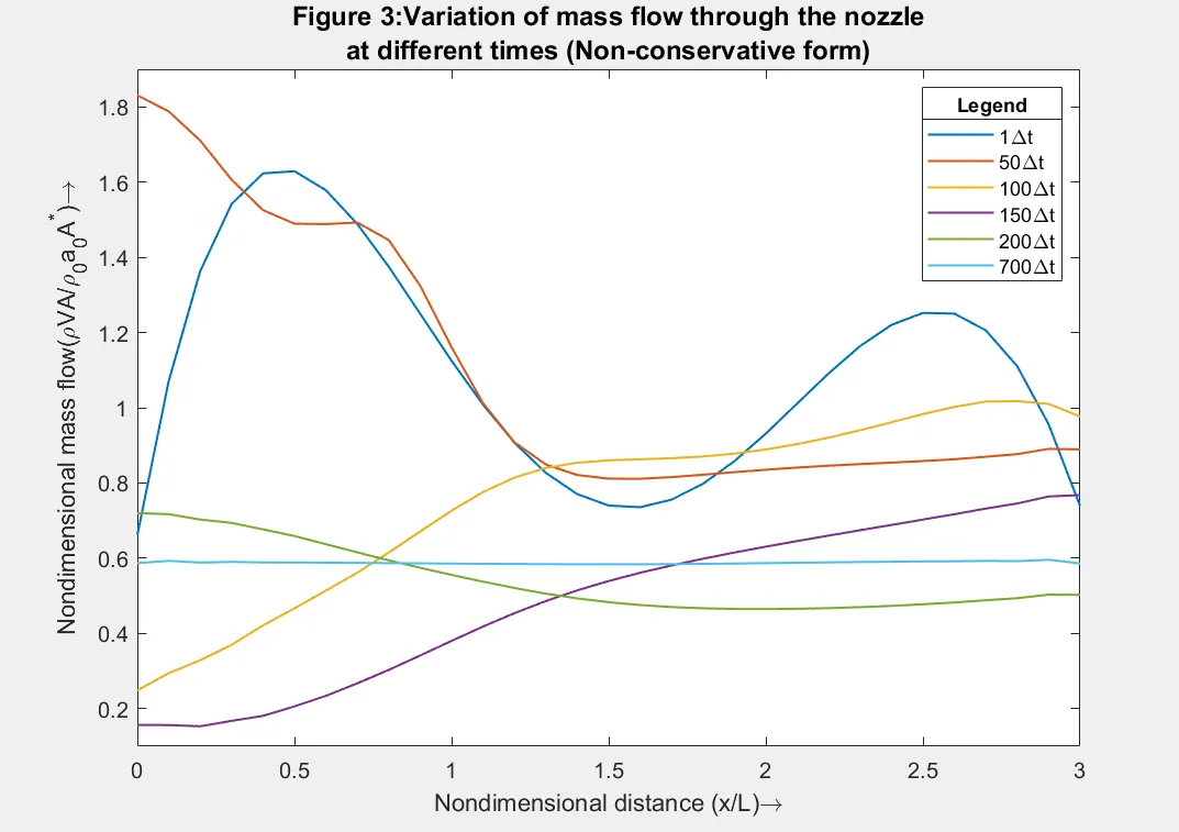
    figure(3)
    plot(x,mnc_call,'linewidth',1.0);
    axis([0 3 0.1 1.9]);
    legendcell = strcat(string(mncplot(1:6)),"\Deltat");
    legend(legendcell,'location','northeast');
    leg=legend('show');
    title(leg,'Legend');
    title({'Figure 3:Variation of mass flow through the nozzle'; 'at different times (Non-conservative form)'},'FontSize',12);
    xlabel('Nondimensional distance (x/L)\rightarrow');
    ylabel('Nondimensional mass flow(\rhoVA/\rho_0a_0A^*)\rightarrow');
end

Plots:

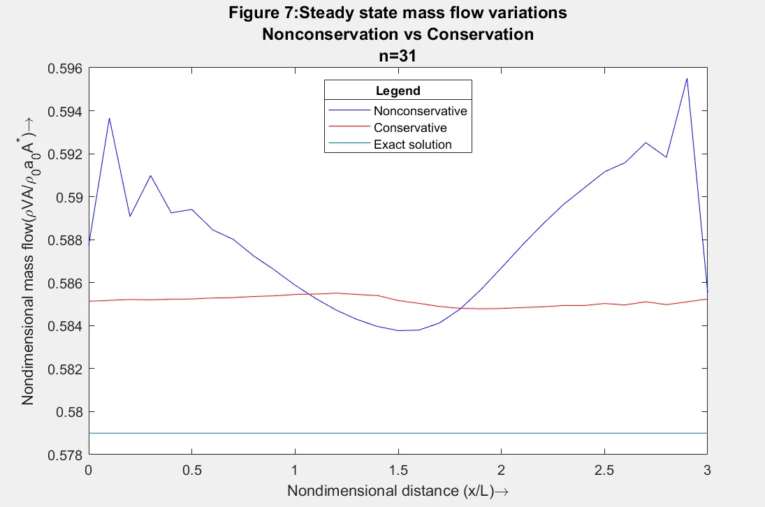
Grid independence check:

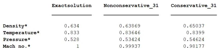
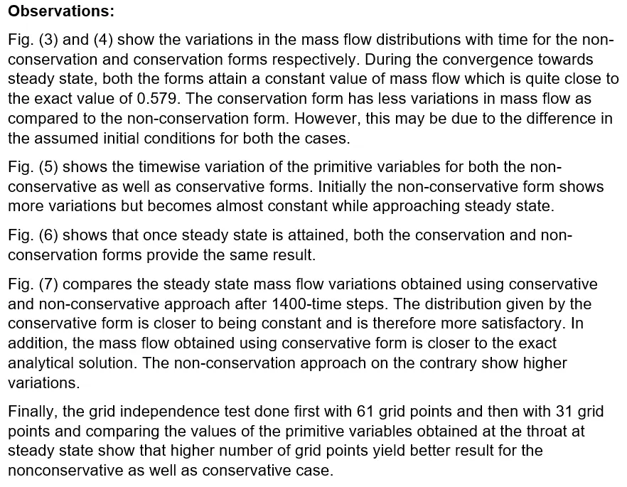
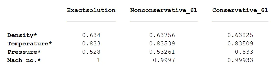
The grid independence test is performed by comparing the values of the dimensionless primitive variables

obtained at the throat of the nozzle by changing the number of nodes as 61 and 31.

The results obtained are as shown below:

For n=61

For n=31