Week 9 - FVM Literature Review
The process of obtaining the computational solution consists of two stages. The first stage involves the conversion of the partial differential equations and auxiliary (boundary and initial) conditions into a system of discrete algebraic equations. This first stage is commonly known as the discretization stage. All numerical methods in the mainstream of CFD to solve the fluid flow equations require some form of discretization. The popular methods are – finite element method (FEM), finite difference method (FDM) and finite volume method (FVM).
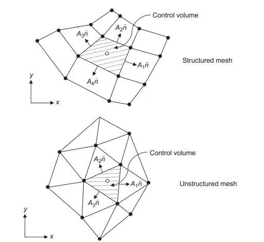
Finite Volume Method –The finite-volume method discretizes the integral form of the conservation equations directly in the physical space. It works with control volumes and not the grid intersection points, it has the capacity to accommodate any type of grid. Here, instead of structured grids, unstructured grids can be employed that allow a large number of options for the definition of the shape and location of the control volumes. Since the grid defines only the control volume boundaries, the method is conservative so long as the surface integrals that are applied at these boundaries are the same as the control volumes sharing the boundary.
Representation of structured and unstructured mesh for the finite-volume method -
The difference between FVM and FDM–
With the finite-difference method, a numerical grid must be initially defined to discretize the physical flow domain of interest. For the finite-volume method, we now have the flexibility of representing the grid by either structured or unstructured mesh. One disadvantage of FVM compared with the finite-difference schemes is that higher-order differencing approximations greater than the second order are more difficult to develop in three dimensions. This is because of the requirement for two levels of approximation, which are interpolation and integration. However, the finite-volume method has more advantages than disadvantages. One important feature of the method is that a ‘finite-element’-type mesh can be used, which the mesh can be formed by the combination of triangles or quadrilaterals in the case of two dimensions or tetrahedra and hexahedra in three dimensions. This type of unstructured mesh offers greater flexibility for handling complex geometries. Another attractive feature is the method requires no transformation of the equations in terms of body-fitted coordinate system as is required in finite-difference method.
Interpolation Scheme –The algebraic forms of equations governing the fluid flow are usually approximated by the application of finite-difference-type approximations to a finite volume cell in space. At each face of the cell volume, surface fluxes of the transport variables that are required can be determined through different interpolation schemes. Some of the common interpolation schemes are first-order upwind, second-order upwind, second-order central, and quadratic upstream interpolation convective kinetics, that’s why respective to FVM interpolation schemes are important.
Flux limiter – flux limiters are used to avoid the wiggles which occurs with high order discretization scheme due to discontinuities and sharp changes in solution domain. Flux limiter scheme limits the spatial derivative to realistic values. Flux limiters are important to get high order accuracy in sooth flow region and get rid of shocks by using first order scheme.
Example of FVM discretization–
Control Volume for 2D continuity equation –
here –
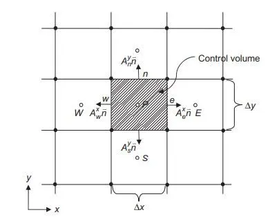
P – centroid
E, W, N, S are the centroids of adjacent control volumes(East, West, North, South)
A is the area with respective to direction and axis
Continuity equation (2D)–

Introducing the control volume integration –
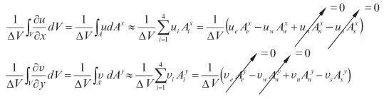
Since the grid has been taken to be uniform, the face velocities u_e, u_w, v_n, and v_s are located midway between each of the control volume centroids, which allows us to determine the face velocities from the values located at the centroids of the control volumes.

substituting the above expressions to the discretized form –

we know –

substituting these values in above written equation –

Simplifying -
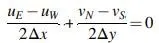
this is the discretized 2D continuity euqation.