Week 9 - FVM Literature Review
Finite Volume Method
Objective:
To understand the Finite Volume Method and the significance of interpolation schemes as well as the flux limiters.
This report is divided into the following sections
- Finite Volume Method introduction
- Interpolation schemes
- Flux Limiters
Finite Volume Method – an Introduction
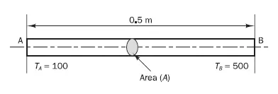
The popularity of the FVM method stems from the fact that the discretization is carried out directly in the physical space without any need for the transformation between physical and computational co-ordinate systems. This enables the FVM method to handle complex geometries with relative ease. This feature can be illustrated with an example. Consider the 1D heat conduction equation
`d/(dx)(k*(dT)/(dx)) + S = 0 `
In Finite Difference Method, the Taylor series is used to discretize the above equation on a grid and it would result in the following equation
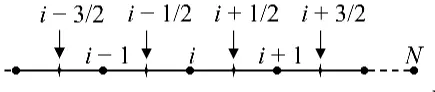
`k*(T_(i-1) – 2*T_i + T_(i+1))/(Deltax^2) + S_i = 0`
The above procedure is repeated for all the nodes in the grid. The resulting algebraic equation will then be solved to obtain solutions at the nodal points.
In Finite Volume Method, the geometry is divided into finite number of control volumes as shown below
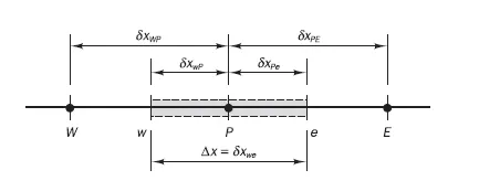
In the above figure, the shaded area represents the control volume and the nodal points are placed at the centre of each control volume. In this method, the governing equation is first integrated within the control volume as follows
`int_(CV) (d/(dx)(k*(dT)/(dx)) dV + int_(CV) S dV = 0 `
This is the step that differentiates FVM from other CFD techniques. Using Gauss-divergence theorem the above equation can be written as
`int_(A) n*(k*(dT)/(dx)) dA + int_(CV) S dV = 0 `
Which on integration over the control volume `P` simplifies into
`k_e *A_e* (dT)/(dx)|_(e) – k_w *A_w* (dT)/(dx)|_(w) + barS*DeltaV = 0 `
Where `e` and `w` are the control volume faces; ` A_e “and” A_w` are the face areas and `barS` is the mean value of the source within the control volume.
As a second step, we use an interpolation scheme to calculate the gradient at the faces. We use the central differencing scheme to determine the value of the gradients as follows
`(dT)/(dx)|_(e) = (T_E – T_P)/(delx_(PE))`
Also interpolation schemes can be used to determine the property values at the faces. Using linear interpolation, we obtain the thermal conductivity as follows:
`k_e = (k_E + k_P)/2`
The source term can be a function of the temperature and it should be linearized. It can be re-written as follows:
`barS*DeltaV = S_u + S_P *T_P`
Therefore, the using the above values, the semi-discretized equation is then converted into fully discretized equation as follows:
`(k_e*A_e*(T_E – T_P)/(delx_(PE)) – k_w*A_w*(T_P – T_W)/(delx_(WP))) + (S_u + S_P *T_P) = 0`
Which on re-arrangement gives
`(k_e/(del_(PE))*A_e + k_w/(delx_(WP))*A_w – S_P)*T_P = (k_e/(del_(PE))*A_e)*T_E + (k_w/(delx_(WP))*A_w) + S_u`
The above equation can be written in terms of co-efficents as follows
`a_PT_P = a_WT_W + a_ET_E + S_u`
Where, `a_P = a_E + a_W – S_P`
The above equation is then applied to all the control volumes within the geometry to obtain a system of algebraic equations which are then solved to obtain the values at the nodal points.
NOTE: On close observation, it can be seen that the discretized equation retains the conservation principle. (i.e) the algebraic sum of net flux through the control volume is equal to the source inside it.
In a similar fashion, the FVM can be extended to 2 and 3 dimensions.
The central differencing approximation used to represent the diffusion terms in the above equation works well for calculating the gradients at the control volume faces. However, the same approach (linear interpolation) can be applied for convective terms where the velocity is required at the faces. In certain cases, such approximation leads to stability and convergence issues [1]. Hence different methods are developed to overcome this issue. Such methods are called interpolation schemes.
Interpolation schemes:
Interpolation schemes are used to transform cell-centre quantities to face centres. Hence such interpolation schemes are important in Finite Volume Method for the calculation of gradient terms. Some of the commonly used interpolation schemes include
- Linear Interpolation or Centre Differencing scheme
- Upwind Differencing scheme
- Hybrid Differencing scheme
- Quadratic Upwind Interpolation Scheme (QUICK)
- TVD interpolation scheme
Linear Interpolation:
In this scheme, the face values are obtained by taking the average of the neighbouring values
`phi_e = (phi_P + phi_E)/2`
Discretization methods using this type of interpolation scheme produce accurate results for diffusion dominated flows and it fails for convection dominated flows. In other words, this scheme works for flows with a Peclet number of less than or equal to 2.
Upwind Differencing Scheme:
The major drawback of the linear interpolation scheme is its inability to detect the flow-direction. The value at the East face `e` is always the average of its neighbouring values. In a strong convective flow from west to east, the above treatment will be unsuitable because the value at face `e` will be strongly influence by node `P` than the value at node `E`.
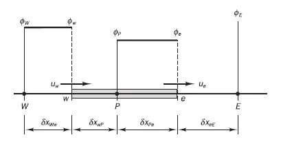
The upwind differencing scheme takes this into consideration and the hence the value at face `e` will always be equal to the value at the upstream node, which in this case will be equal to `phi_P`
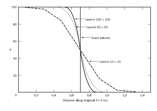
The major drawback of this scheme is that it produces artificial diffusion when the flow is not aligned with the grid lines.
Consider a problem with a uniform rectangular grid as shown below with a flow along its diagonal
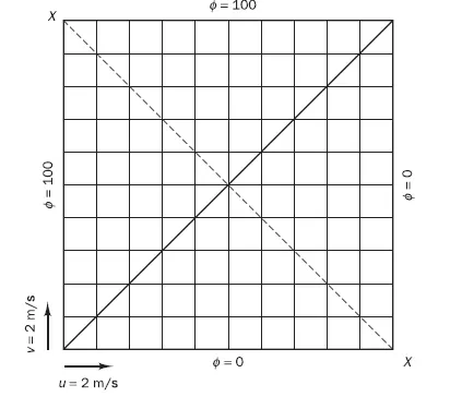
The figure below illustrates this behaviour [1]. It can be observed that more number of grid points are needed to get a more accurate solution. The detailed explanation can be found in [1]
Hybrid Scheme:
The hybrid scheme is a combination of the above two schemes. It uses a piecewise formula based on the local Peclet number to evaluate the net flux through the control volume. For `|Pe| > 2` upwind differencing is used and for `|Pe| < 2` the central differencing scheme is used.
In this way, this scheme is switches to upwind differencing at high `Pe`numbers where the central differencing will produce inaccurate results. ^
The accuracy of the upwind and the hybrid schemes are only first order in terms of taylor truncation error. Hence they are prone to numerical errors. To overcome this, several higher order methods were developed. Some of them include
Quadratic Upwind Interpolation Scheme:
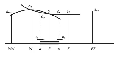
This scheme uses a three point weighted quadratic interpolation to calculate the face values. For example, consider a flow flowing from west to east, then the value at `w` is given by considering a quadratic interpolation among the `phi_P , phi_W and phi_(WW)` Similarly the value at `e` is obtained by utilising the values at `phi_E, phi_P and phi_W`. The weighting for the different values used in this method are shown in the below equation
`phi_w = 6/8 * phi_W + 3/8 * phi_P – 1/8 * phi_(WW)`
This scheme is third-order accurate in terms of taylor truncation error because of the use of quadratic terms. The stability of this scheme depends on local Pe number and therefore it is only conditionally stable.
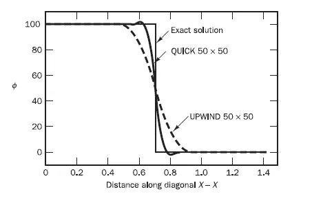
When comparing with the upwind scheme, the QUICK scheme produces more accurate results for non-aligned flows. However, it also produces overshoots and undershoots as it can be observed from the above figure. Therefore, one must be critical when analysing the results obtained from the QUICK scheme.
TVD Scheme:
TVD stands for total variation diminishing and it represent the schemes which produces oscillation free solutions.
Consider a discrete data set as shown in figure
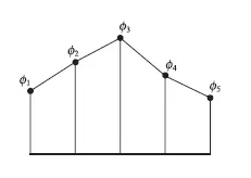
A total variation for such a distribution of data can be represented as
`TV(phi) = | phi_2 – phi_1 | + | phi_3 – phi_2 | + | phi_4 – phi_3 | + | phi_5 – phi_4 |`
When this total variation decreasing with time-step, then the scheme is called Total Variation Diminishing (TVD) scheme.
So far, it has been established that the stable upwind scheme is first order accurate. However, the third-order accurate schemes such as QUICK produce wiggles in the solution. Therefore, an incentive was prevelant to convert the stable first-order accurate upwind scheme to higher order accurate. This is achieved by adding an artificial diffusion or by adding a weighting towards upstream contribution.
In general the TVD schemes can be written as
For a east face value
`phi_e = phi_P + ½* psi(r)*(phi_E-phi_P)`
Where psi(r) is called a flux limiter function to limit the influence of additional upstream convective flux (`phi_E – phi_P`) which was added to convert the upwind scheme into higher order.
`psi` is a function of r which is the ratio of upwind-side gradient to the downwind-side gradient. For a east face, the value of r is as follows
`r= (phi_P -phi_W)/(phi_P -phi_E)`
Flux limiter function:
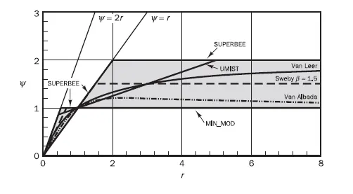
It is important to note that all the above schemes can be represented as the upwind scheme with an extra gradient term added to it. The influence of this extra gradient term varies depending on the individual scheme and this influence is implemented through the `psi` function. When `psi(r) = 1`, we obtain the central differencing scheme and when `psi(r) = 0`, we obtain the upwind-differencing scheme.
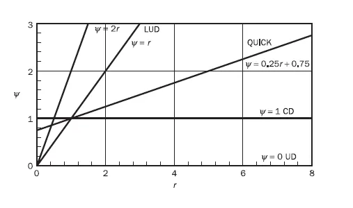
Sweby [2] has given the necessary and sufficient conditions in terms flux-limiter function for a scheme to be TVD. In the following figure, the shaded area represents the Sweby conditions for the flux-limiter functions for a second-order accurate discretization schemes. It also shows different flux-limiter functions that are available in the literature.
Acknowledgement:
The figures and the comparisons of different schemes are obtained from the book “An introduction to Computational Fluid Dynamics: The Finite Volume Method “ by H K Versteeg
References:
- Versteeg, Henk Kaarle, and Weeratunge Malalasekera. An introduction to computational fluid dynamics: the finite volume method. Pearson education, 2007.
- Sweby, Peter K. "High resolution schemes using flux limiters for hyperbolic conservation laws." SIAM journal on numerical analysis5 (1984): 995-1011.