Week 8 - Simulation of a backward facing step in OpenFOAM

Case Setup in OpenFOAM

1. Starting with the Reference Case:

We will base this simulation on the forwardStep case from the OpenFOAM tutorials ($FOAM_TUTORIALS/incompressible/simpleFoam/forwardStep). Since this is a transient simulation with a laminar flow model, we'll modify the case accordingly.

2. Domain Setup:

The geometry is a backward-facing step. The domain length is 1 m in the x-direction, the height upstream of the step is 0.2 m, and downstream of the step, it is 0.3 m. The step is located at x = 0.0 m and has a height of 0.1 m. The figure defines the geometry and boundary conditions.

Create the following directories if not already present:

• system/: For numerical methods and control files.
• constant/: For physical properties.
• 0/: For initial and boundary conditions.

3. Geometry and Mesh Generation:

To simulate the flow, we will define the mesh parameters based on the problem specifications. We will first create a structured mesh and then introduce the grading factor (GF) for Case 2.

In Case 1, simpleGrading is set to (1 1 1) for uniform mesh, while in Case 2, the grading is applied in the y-direction (i.e., finer near walls and the step).

4. Boundary Conditions:

• Inlet: Constant velocity inlet (chosen to keep the flow laminar).
• Outlet: Zero gradient for pressure and velocity.
• Walls: No-slip boundary condition (velocity is zero).

5. Solver Selection:

Since this is an incompressible, laminar, viscous flow, we will use the pimpleFoam solver. This solver handles transient incompressible flow problems.

6. Turbulence Model:

We will switch off turbulence since we are dealing with laminar flow. In constant/turbulenceProperties, set:

7. Time Controls:

In system/control Dict, set up the time step:

MATLAB Code for Mesh Specification

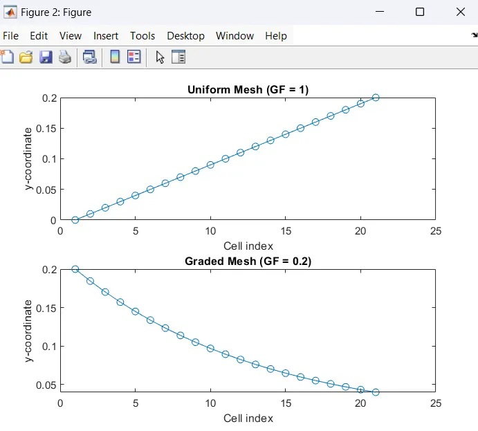
For generating a mesh with a grading factor, we will first write MATLAB code to compare mesh generation for both cases.

MATLAB Code for Mesh Generation:

% Parameters for mesh

Lx = 1; % length of domain in x-direction (m)

Ly1 = 0.2; % height before the step

Ly2 = 0.3; % height after the step

Nx = 200; % Number of cells in x-direction

Ny1 = 20; % Number of cells in y-direction (before step)

Ny2 = 20; % Number of cells in y-direction (after step)

% Case 1: No grading factor (GF = 1)

GF1 = 1;

dy_uniform = linspace(0, Ly1, Ny1+1); % Uniform grid before step

dy_uniform_step = linspace(0, Ly2, Ny2+1); % Uniform grid after step

% Case 2: With grading factor (GF = 0.2)

GF2 = 0.2;

dy_graded = Ly1 * (GF2 .^ ((0:Ny1) / Ny1)); % Graded grid before step

dy_graded_step = Ly2 * (GF2 .^ ((0:Ny2) / Ny2)); % Graded grid after step

% Plotting the mesh

figure;

subplot(2,1,1);

plot(dy_uniform, 'o-');

title('Uniform Mesh (GF = 1)');

ylabel('y-coordinate');

xlabel('Cell index');

subplot(2,1,2);

plot(dy_graded, 'o-');

title('Graded Mesh (GF = 0.2)');

ylabel('y-coordinate');

xlabel('Cell index');

Case Studies and Comparison of Results

Case 1: Simulation without a grading factor (GF = 1)

• Mesh: Uniform.
• Velocity profile at x = 0.085 m measured and plotted using Paraview's "Plot Over Line" tool.

Case 2: Simulation with a grading factor (GF = 0.2)

• Mesh: Finer cells near the walls and step due to grading.
• Velocity profile at x = 0.085 m measured and compared to Case 1.

Importance of Grading Factor in Meshing

Grading/Growth factor is essential in meshing because:

1. Accuracy near walls: In boundary layer flows, finer meshes are required near walls to capture the velocity gradient and viscous effects more accurately.
2. Computational efficiency: Grading allows you to concentrate the mesh resolution where it is needed (e.g., near walls) while coarsening the mesh in regions with less variation (e.g., the core flow), reducing the computational cost.
3. Capturing Flow Details: In complex geometries such as the backward-facing step, a finer mesh near the step helps capture flow separation and reattachment zones accurately.