Week 8 - Simulation of a backward facing step in OpenFOAM
Simulation of backwards-facing step in OpenFOAM
Aim:
To simulate a transient incompressible laminar flow through a backward-facing step geometry using OpenFOAM
Objectives:
The backward-facing step problem is a well-known academic problem for studying the internal flows. The main objective of solving this problem is to learn the process of simulating a case in openFOAM from setting up the case till post-processing the obtained solution.
Introduction:
The dimensions of the backward-facing step geometry used in this project is shown below
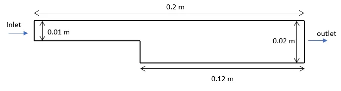
The backward-facing step is one of the representative models for the separation flows which can be widely observed in various applications such as airfoils, cars, boats and even flow around buildings. Because of the sudden increase in area, the flow is separated from the boundary and it again reattaches further downstream. It is one of the benchmarked geometries and it is widely used in the study of numerical CFD.
Methodology:
Step 1: Selection of suitable solver
OpenFOAM has a wide variety of solvers for specific use-cases. Based on the requirement, one has to be selected. In this report, the physics being solved is the flow of incompressible viscous laminar flow. The suitable solver for such a case is icoFOAM.
Step 2: Setting up the case
OpenFOAM, being an open-source software lacks a graphical user interface. Therefore, the case has to be set up using the folder structure inherent to it. As a beginner, the best approach is to copy a tutorial case that uses the required solver and change the settings as required.
The cavity tutorial, which uses the icoFOAM solver was copied for this report.
Step 3: Creating a mesh
Once the folder structure is set up, the mesh for the geometry has to be generated. For this purpose, blockMesh, the inherent feature of OpenFOAM was used. The blockMesh requires the definition of rectangular blocks within the geometry and hence the geometry was split into 3 blocks as shown below. First, the vertices should be defined and then the blocks should be created from the vertices such that the local coordinated system of the block is the same.
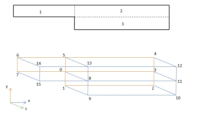
OpenFOAM is a 3D solver and therefore blocks should also be 3D. Hence the blocks were created based on the configuration shown above. A 2D case can be simulated by specifying a single cell in the z-direction. In addition to the blocks, the number of cells and the grading should be defined for each block. The configuration used in this project is summarized in the following table
Number of cells in each block along a particular direction
|
Blocks |
x-direction |
y-direction |
z-direction |
|
1 |
80 |
10 |
1 |
|
2 |
120 |
10 |
1 |
|
3 |
120 |
10 |
1 |
Two variations of the same case were simulated. In the first case, no grading was used in the mesh. In the second one, a grading of 0.2 was used and the results were compared.
Grading is a term used to defined the relative size of the last cell in a block with respect to the first cell.
The above parameters should be defined in the file, blockMeshDict inside the settings folder. The blockMeshDict file used in this simulation is shown below
/*--------------------------------*- C++ -*----------------------------------*\
  =========                 |
  \\      /  F ield         | OpenFOAM: The Open Source CFD Toolbox
   \\    /   O peration     | Website:  https://openfoam.org
    \\  /    A nd           | Version:  6
     \\/     M anipulation  |
\*---------------------------------------------------------------------------*/
FoamFile
{
    version     2.0;
    format      ascii;
    class       dictionary;
    object      blockMeshDict;
}
// * * * * * * * * * * * * * * * * * * * * * * * * * * * * * * * * * * * * * //

convertToMeters 0.01;

vertices
(
// Back plane
    (0 0 0)
    (0 -1 0)
    (12 -1 0)
    (12 0 0)
    (12 1 0)
    (0 1 0)
    (-8 1 0)
    (-8 0 0)

// Front Plane
    (0 0 0.1)
    (0 -1 0.1)
    (12 -1 0.1)
    (12 0 0.1)
    (12 1 0.1)
    (0 1 0.1)
    (-8 1 0.1)
    (-8 0 0.1)


);

blocks
(
//block 1
    hex (7 0 5 6 15 8 13 14) (80 10 1) simpleGrading (1 1 1)

//block 2
    hex (0 3 4 5 8 11 12 13) (120 10 1) simpleGrading (1 1 1)

//block 3
    hex (1 2 3 0 9 10 11 8) (120 10 1) simpleGrading (1 1 1)

);

edges
(
);

boundary
(
    inlet
    {
        type patch;
        faces
        (
            (7 15 14 6)
        );
    }
    outlet
    {
        type patch;
        faces
        (
            (3 4 12 11)
            (2 3 11 10)
        );
    }
    upperWall
    {
        type wall;
        faces
        (
            (6 14 13 5)
            (5 13 12 4)
        );
    }
    lowerWall
    {
        type wall;
        faces
        (
            (7 0 8 15)
            (1 2 10 9)
            (0 1 9 8)
        );
    }
    frontAndBack
    {
        type empty;
        faces
        (
            (14 15 8 13)
            (13 8 11 12)
            (8 9 10 11)
            (6 5 0 7)
            (5 4 3 0)
            (0 3 2 1)
        );
    }
);

// ************************************************************************* //
The boundary faces should also be defined in the blockMeshDict along with a unique for each boundary. In the above file, the boundaries defined are inlet, outlet, upperWall, lowerWall and frontAndBack. All the faces exhibiting a similar boundary condition can be grouped under a single boundary name.
For grading, the following lines were changed in the above file
blocks
(
//block 1
    hex (7 0 5 6 15 8 13 14) (80 10 1) simpleGrading (0.2 5 1)

//block 2
    hex (0 3 4 5 8 11 12 13) (120 10 1) simpleGrading (5 5 1)

//block 3
    hex (1 2 3 0 9 10 11 8) (120 10 1) simpleGrading (5 0.2 1)

);
Step 4: initial condition
Next, the initial conditions should be defined. These conditions can be defined in the 0 folder for each variable. The variables solved in this case are velocity and pressure and each variable has a separate file inside the 0 folder. These files are shown below along with the value used.
Velocity:
/*--------------------------------*- C++ -*----------------------------------*\
  =========                 |
  \\      /  F ield         | OpenFOAM: The Open Source CFD Toolbox
   \\    /   O peration     | Website:  https://openfoam.org
    \\  /    A nd           | Version:  6
     \\/     M anipulation  |
\*---------------------------------------------------------------------------*/
FoamFile
{
    version     2.0;
    format      ascii;
    class       volVectorField;
    object      U;
}
// * * * * * * * * * * * * * * * * * * * * * * * * * * * * * * * * * * * * * //

dimensions      [0 1 -1 0 0 0 0];

internalField   uniform (0 0 0);

boundaryField
{
    inlet
    {
        type            fixedValue;
        value           uniform (1 0 0);
    }

    outlet
    {
        type            zeroGradient;
    }

    upperWall
    {
        type            noSlip;
    }

    lowerWall
    {
        type            noSlip;
    }

    frontAndBack
    {
        type            empty;
    }
}

// ************************************************************************* //
Pressure file:
FoamFile
{
    version     2.0;
    format      ascii;
    class       volScalarField;
    object      p;
}
// * * * * * * * * * * * * * * * * * * * * * * * * * * * * * * * * * * * * * //

dimensions      [0 2 -2 0 0 0 0];

internalField   uniform 0;

boundaryField
{
    inlet
    {
        type            zeroGradient;
    }

    outlet
    {
        type            fixedValue;
	value		uniform 0;
    }

    upperWall
    {
        type            zeroGradient;
    }

    lowerWall
    {
        type            zeroGradient;
    }

    frontAndBack
    {
        type            empty;
    }
}

// ************************************************************************* //
Step 5: Specification of transport properties
Since this is a viscous flow, the co-efficient of viscosity should be defined. This is a constant property and hence was defined in transportProperties within the constant folder. A value of 1.56e-5 (kinematic viscosity of air) was used here.
Step 6: Specification of Simulation controls:
Finally, the simulation controls should be defined. The simulation control include, endtime, time-step size, etc. The time-discretization used here was the explicit method and hence a time-step size based on courant number should be used. According to the CFL condition,
`Deltat = 1*(Deltax)/V`
Where V is the initial velocity
In this case, a `Deltat` value of 0.0005 s was chosen which satisfied the CFL condition.
The controlDict file used in the project is shown below:
/*--------------------------------*- C++ -*----------------------------------*\
  =========                 |
  \\      /  F ield         | OpenFOAM: The Open Source CFD Toolbox
   \\    /   O peration     | Website:  https://openfoam.org
    \\  /    A nd           | Version:  6
     \\/     M anipulation  |
\*---------------------------------------------------------------------------*/
FoamFile
{
    version     2.0;
    format      ascii;
    class       dictionary;
    location    "system";
    object      controlDict;
}
// * * * * * * * * * * * * * * * * * * * * * * * * * * * * * * * * * * * * * //

application     icoFoam;

startFrom       startTime;

startTime       0;

stopAt          endTime;

endTime         0.8;

deltaT          0.0005;

writeControl    timeStep;

writeInterval   20;

purgeWrite      0;

writeFormat     ascii;

writePrecision  6;

writeCompression off;

timeFormat      general;

timePrecision   6;

runTimeModifiable true;


// ************************************************************************* //
In the end, the simulation was ran using the following commands
>> blockMesh
To generate the mesh
>> icoFoam
To run the solver
>> paraFoam
To open the post-processing
The post-processing was done using Paraview, which is also an open source program.
Results:
Mesh grading = 1 (no mesh grading)
The mesh generated is as follows:
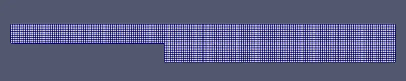
It can be observed that the mesh is uniformly sized everywhere.
The simulation was performed for a total time of 0.8 s. At the end of the simulation, the velocity distribution was obtained as follows
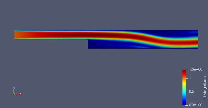
It can be observed that the flow separates at the step and it reattaches downstream. As a comparison, the velocity profile along the y-axis was plotted at a distance of 0.085 m from the inlet. This location was 0.005 m from the step. The following velocity profile was obtained at the location
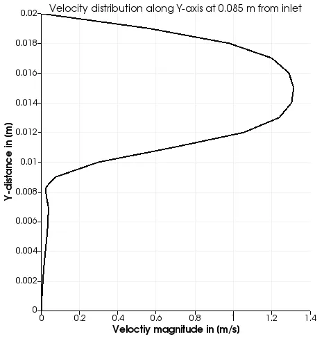
Because of the recirculation, the velocity below the step is very low.
Mesh grading = 0.2
The mesh generated for this case is as follows:
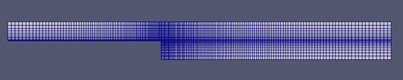
Because of the grading, the mesh size is low near the wall and it is comparatively large at the other end. One thing to note is that the number of cells is the same as in the previous case.
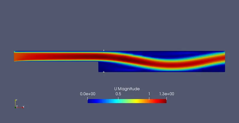
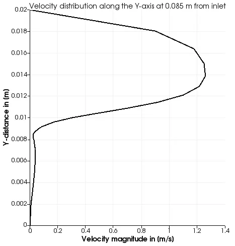
The contour plot and the velocity profile obtained are as follows:
Conclusion:
With mesh grading, the flow quantities were calculated at more grid points near the wall. Hence the resolution of velocity with the mesh-grading is more accurate than without grading.
Similarly, having more number of grid points near the walls, the point of reattachment can be captured accurately