Simulation of a Backward Facing Step in OpenFOAM
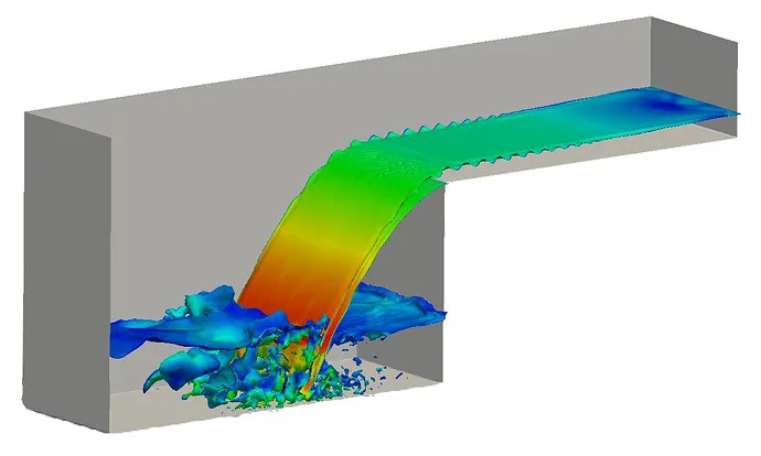
To simulate a Transient Incompressible-Laminar-Viscous flow through the backwards-facing step geometry transient simulation
Transient Incompressible-Laminar-Viscous Flow
Incompressible Flow
Incompressible flow refers to a flow in which the density remains constant in any fluid parcel, i.e. any infinitesimal volume of fluid moving in the flow. This type of flow is also referred to as isochoric flow.
An equivalent statement that implies incompressibility is that the divergence of the flow velocity is zero (see the derivation below, which illustrates why these conditions are equivalent).
Incompressible flow does not imply that the fluid itself is incompressible. It is shown in the derivation below that (under the right conditions) even compressible fluids can – to a good approximation – be modelled as an incompressible flow. Incompressible flow implies that the density remains constant within a parcel of fluid that moves with the flow velocity.
Example
The most common example is the simulation of liquid flows — especially water, due to its high bulk modulus.
Inviscid and Viscous Flow
Inviscid flow is the flow of an inviscid fluid, in which the viscosity of the fluid is equal to zero. Though there are limited examples of inviscid fluids, known as superfluids, the inviscid flow has many applications in fluid dynamics. The Reynolds number of inviscid flow approaches infinity as the viscosity approaches zero. It is assumed the region of fluid near a solid boundary offers negligible viscosity.
The fluid itself need not have zero viscosity for inviscid flow to occur. It is also possible to arrange the flow of a viscous fluid so that viscous forces vanish. Such a flow has no viscous resistance to its motion.
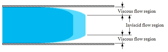
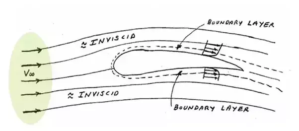
The development of viscous and inviscid regions of flow as a result of inserting a flat plate parallel into a fluid stream of uniform velocity is shown. The fluid sticks to the plate on both sides because of the no-slip condition, and the thin boundary layer in which the viscous effects are significant near the plate surface is the viscous flow region. The region of flow on both sides away from the plate and unaffected by the presence of the plate is the inviscid flow region.
Laminar Flow
Laminar flow is characterized by fluid particles following smooth paths in layers, with each layer moving smoothly past the adjacent layers with little or no mixing. At low velocities, the fluid tends to flow without lateral mixing, and adjacent layers slide past one another. There are no cross-currents perpendicular to the direction of flow, nor eddies or swirls of fluids. In laminar flow, the motion of the particles of the fluid is very orderly with particles close to a solid surface moving in straight lines parallel to that surface.
The laminar regime is ruled by momentum diffusion, while the momentum convection is less important. In more physical terms, it means that viscous forces are higher than inertial forces.
(a) Laminar flow in a closed pipe, (b) Turbulent flow in a closed pipe. The laminar region is smooth with less chaos because the turbulent flow has high momentum convection.
Setting Up the case in OpenFOAM
An OpenFOAM case requires definitions for the mesh, initial fields, physical models, control parameters, etc.
Step-1 Preprocessing
Pre-processing
- Definition of the geometry of the region of interest: the computational domain
- Grid generation – the sub-division of the flow region into a number of smaller, non-overlapping sub-domains: a grid (or mesh) of cells (or control volumes or elements)
- Selection of suitable models for the interesting physical and chemical
phenomena - Definition of fluid properties
- Specification of the appropriate chemical and physical boundary conditions at cells that coincide with or touch the domain boundary
The solution to a flow problem (velocity, pressure, temperature etc.) is defined at
nodes or cell centres inside each cell. The accuracy of a CFD solution depends heavily on the number of cells in the grid. In general, the larger the number of cells, the better the solution accuracy. Optimal meshes are often non-uniform: finer in areas where large variations occur from point to point and coarser in regions with relatively little change.
Solving
There are at least four distinct streams of numerical solution techniques: finite
the difference, finite element, spectral methods and finite volume. We will only focus on
the finite volume method, as it is central to the most well-established CFD solvers. In outline, the finite volume method consists of the following steps:
- Integration of the conservation of mass, energy and momentum equations over all the control volumes in the domain
- Discretization – conversion of the resulting integral equations into a system of algebraic equations
- Solution of the algebraic equations by an iterative method
The first step, the control volume integration, makes the finite volume method
different from all other CFD techniques. It makes sure that a general flow variable, e.g. momentum or enthalpy is conserved in each finite-size cell. This clear relationship between the numerical algorithm and the underlying conservation principle makes the finite volume method popular and much simpler to understand.
Post-processing
This is where you take a look at the results and visualize them so that you can see
what happens in your model. Typical elements of post-processing are:
- Definition of suitable cutting planes for visualization
- Contour plots of properties/flow variables
- Vector plots
- Streamlines
- Line plots
- Balances
Given Geometry
Case 1 - Simulate the flow without using any grading factor (i.e., GF = 1)
The simple description specifies uniform expansions in the local `x`, `y` and `z` directions respectively with only 3 expansion ratios.
Grading Factor= (size of end cell) / (size of starting cell)
Creating the geomtery by editing editing the blockMeshDict File
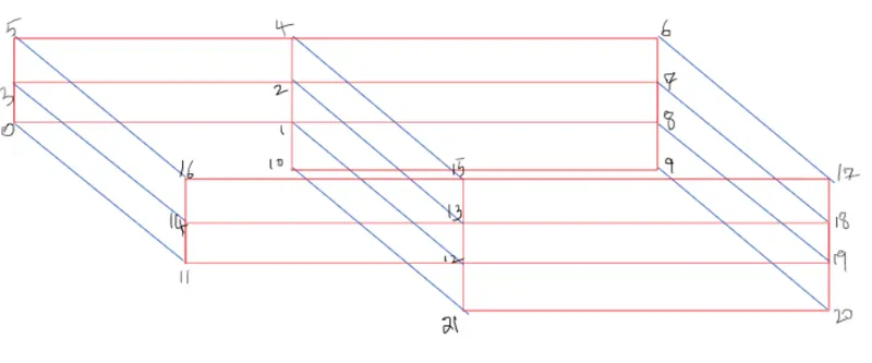
Edited blockMeshDict
To edit the blockMeshDict file we first declare all the vertices as points which all then used to determine the vertices of blocks. The block are created using the vertices and the no. of elements are defined in `x`, `y` and `z` direction is defined along with the grading. After this we define boundary condition using the faces of the blocks, that is the inlet, outlet, upper walls, lower walls, front and back.
/*--------------------------------*- C++ -*----------------------------------*
  =========                 |
  \      /  F ield         | OpenFOAM: The Open Source CFD Toolbox
   \    /   O peration     | Website:  https://openfoam.org
    \  /    A nd           | Version:  8
     \/     M anipulation  |
*---------------------------------------------------------------------------*/
FoamFile
{
    version     2.0;
    format      ascii;
    class       dictionary;
    object      blockMeshDict;
}
// * * * * * * * * * * * * * * * * * * * * * * * * * * * * * * * * * * * * * //

convertToMeters 1;

vertices
(
    (0 0 0)			//Point 0
    (0.08 0 0)			//Point 1
    (0.08 0.005 0)		//Point 2
    (0 0.005 0)		        //Point 3
    (0.08 0.01 0)		//Point 4
    (0 0.01 0)			//Point 5
    (0.2 0.01 0)		//Point 6
    (0.2 0.005 0)		//Point 7
    (0.2 0 0)			//Point 8
    (0.2 -0.01 0)		//Point 9
    (0.08 -0.01 0)		//Point 10
    (0 0 0.001)		        //Point 11
    (0.08 0 0.001)		//Point 12
    (0.08 0.005 0.001)		//Point 13
    (0 0.005 0.001)		//Point 14
    (0.08 0.01 0.001)		//Point 15
    (0 0.01 0.001)		//Point 16
    (0.2 0.01 0.001)		//Point 17
    (0.2 0.005 0.001)		//Point 18
    (0.2 0 0.001)		//Point 19
    (0.2 -0.01 0.001)		//Point 20
    (0.08 -0.01 0.001)		//Point 21
);

blocks
(
    hex (0 1 2 3 11 12 13 14)
    (80 5 1)
    simpleGrading (1 1 1)

    hex (3 2 4 5 14 13 15 16)
    (80 5 1)
    simpleGrading (1 1 1)

    hex (2 7 6 4 13 18 17 15)
    (120 5 1)
    simpleGrading (1 1 1)

    hex (1 8 7 2 12 19 18 13)
    (120 5 1)
    simpleGrading (1 1 1)

    hex (10 9 8 1 21 20 19 12)
    (120 10 1)
    simpleGrading (1 1 1)
);

edges
(
);

boundary
(
    inlet
    {
        type patch;
        faces
        (
            (0 11 14 3)
            (3 14 16 5)
        );
    }
    outlet
    {
        type patch;
        faces
        (
            (7 6 17 18)
            (8 7 18 19)
            (9 8 19 20 )
        );
    }
    upperWall
    {
        type wall;
        faces
        (
            (16 15 4 5)
            (15 17 6 4)
        );
    }
    lowerWall
    {
        type wall;
        faces
        (
            (0 1 12 11)
            (10 9 20 21)
            (10 21 12 1)
        );
    }
    frontAndBack
    {
        type empty;
        faces
        (
            (11 12 13 14)
            (14 13 15 16)
            (21 20 19 12)
            (12 19 18 13)
            (13 18 17 15)
            (0 3 2 1)
            (3 5 4 2)
            (2 4 6 7)
            (1 2 7 8)
            (10 1 8 9)
        );
    }
);

mergePatchPairs
(
);

// ************************************************************************* //
Running blockMesh to using paraFoam to view the generated mesh

Updating Initial Condition in Folder 0
Initial velocity
The velocity at the inlet is specified and the at the outlet is specified as a gradient. The unit for velocity is specified using the 7 primary dimensions. As the flow is viscous we specify no-slip condition.
/*--------------------------------*- C++ -*----------------------------------*
  =========                 |
  \      /  F ield         | OpenFOAM: The Open Source CFD Toolbox
   \    /   O peration     | Website:  https://openfoam.org
    \  /    A nd           | Version:  8
     \/     M anipulation  |
*---------------------------------------------------------------------------*/
FoamFile
{
    version     2.0;
    format      ascii;
    class       volVectorField;
    object      U;
}
// * * * * * * * * * * * * * * * * * * * * * * * * * * * * * * * * * * * * * //

dimensions      [0 1 -1 0 0 0 0];

internalField   uniform (0 0 0);		//Initial Condition

boundaryField
{
    inlet
    {
        type            fixedValue;
        value           uniform (0.1 0 0);		//Velocity at inlet
    }

    outlet
    {
        type            zeroGradient;			//Velocity at outlet
    }

    upperWall
    {
        type            noSlip;			//Viscous Flow
    }

    lowerWall
    {
        type            noSlip;			//Viscous Flow
    }

    frontAndBack
    {
        type            empty;			//Boundary in z-direction is considered as infinite
    }
}

// ************************************************************************* //
Initial Pressure
The pressure at the inlet is not known and we specify is in form of a gradient. The outlet pressure is set to zero as the outlet pressure is the same as the atmosphere and the gauge pressure reading will be zero.
/*--------------------------------*- C++ -*----------------------------------*
  =========                 |
  \      /  F ield         | OpenFOAM: The Open Source CFD Toolbox
   \    /   O peration     | Website:  https://openfoam.org
    \  /    A nd           | Version:  8
     \/     M anipulation  |
*---------------------------------------------------------------------------*/
FoamFile
{
    version     2.0;
    format      ascii;
    class       volScalarField;
    object      p;
}
// * * * * * * * * * * * * * * * * * * * * * * * * * * * * * * * * * * * * * //

dimensions      [0 2 -2 0 0 0 0];

internalField   uniform 0;		//Initial Condition

boundaryField
{
    inlet
    {
        type            zeroGradient;
    }

    outlet
    {
        type            fixedValue;
        value           uniform 0;
    }

    upperWall
    {
        type            zeroGradient;
    }

    lowerWall
    {
        type            zeroGradient;
    }

    frontAndBack
    {
        type            empty;
    }
}

// ************************************************************************* //
Updating transport properties in constant folder
Based on the fluid the fluid properties are specified in the transport properties file. Here we assume the fluid to be air.
/*--------------------------------*- C++ -*----------------------------------*
  =========                 |
  \      /  F ield         | OpenFOAM: The Open Source CFD Toolbox
   \    /   O peration     | Website:  https://openfoam.org
    \  /    A nd           | Version:  8
     \/     M anipulation  |
*---------------------------------------------------------------------------*/
FoamFile
{
    version     2.0;
    format      ascii;
    class       dictionary;
    location    "constant";
    object      transportProperties;
}
// * * * * * * * * * * * * * * * * * * * * * * * * * * * * * * * * * * * * * //

nu              [0 2 -1 0 0 0 0] 1.48e-5;	//viscosity of air


// ************************************************************************* //
Runtime and Timestep
Until now we have specified all the initial, boundary and fluid properties for the simulation setup. The staring and the ending time of the simulation along with the timestep are entered in the controlDict in the system folder.
The total time for the simulation is estimated on the basis of the domain length and how fast the information is travelling in the domain, and the time step is estimated using the CFL number based on the stability of the governing equation.
Edited controlDict file
/*--------------------------------*- C++ -*----------------------------------*
  =========                 |
  \      /  F ield         | OpenFOAM: The Open Source CFD Toolbox
   \    /   O peration     | Website:  https://openfoam.org
    \  /    A nd           | Version:  8
     \/     M anipulation  |
*---------------------------------------------------------------------------*/
FoamFile
{
    version     2.0;
    format      ascii;
    class       dictionary;
    location    "system";
    object      controlDict;
}
// * * * * * * * * * * * * * * * * * * * * * * * * * * * * * * * * * * * * * //

application     icoFoam;

startFrom       startTime;

startTime       0;

stopAt          endTime;

endTime         2;

deltaT          0.001;

writeControl    timeStep;

writeInterval   1;

purgeWrite      0;

writeFormat     ascii;

writePrecision  6;

writeCompression off;

timeFormat      general;

timePrecision   6;

runTimeModifiable true;


// ************************************************************************* //
Case 2 - Simulate the flow with a grading factor of 0.2. The cells should be finer near the walls (including the step wall).
The case-2 setup remains same as case-1 but inorder to have finer cells we use the grading option available in the blockMesh
/*--------------------------------*- C++ -*----------------------------------*
  =========                 |
  \      /  F ield         | OpenFOAM: The Open Source CFD Toolbox
   \    /   O peration     | Website:  https://openfoam.org
    \  /    A nd           | Version:  8
     \/     M anipulation  |
*---------------------------------------------------------------------------*/
FoamFile
{
    version     2.0;
    format      ascii;
    class       dictionary;
    object      blockMeshDict;
}
// * * * * * * * * * * * * * * * * * * * * * * * * * * * * * * * * * * * * * //

convertToMeters 1;

vertices
(
    (0 0 0)			//0
    (0.08 0 0)			//1
    (0.08 0.005 0)		//2
    (0 0.005 0)		//3
    (0.08 0.01 0)		//4
    (0 0.01 0)			//5
    (0.2 0.01 0)		//6
    (0.2 0.005 0)		//7
    (0.2 0 0)			//8
    (0.2 -0.01 0)		//9
    (0.08 -0.01 0)		//10
    (0 0 0.001)		//11
    (0.08 0 0.001)		//12
    (0.08 0.005 0.001)		//13
    (0 0.005 0.001)		//14
    (0.08 0.01 0.001)		//15
    (0 0.01 0.001)		//16
    (0.2 0.01 0.001)		//17
    (0.2 0.005 0.001)		//18
    (0.2 0 0.001)		//19
    (0.2 -0.01 0.001)		//20
    (0.08 -0.01 0.001)		//21
);

blocks
(
    hex (0 1 2 3 11 12 13 14)
    (80 5 1)
    simpleGrading (1 5 1)		//Grading

    hex (3 2 4 5 14 13 15 16)
    (80 5 1)
    simpleGrading (1 0.2 1)		//Grading

    hex (2 7 6 4 13 18 17 15)
    (120 5 1)
    simpleGrading (5 0.2 1)		//Grading

    hex (1 8 7 2 12 19 18 13)
    (120 5 1)
    simpleGrading (5 5 1)		//Grading

    hex (10 9 8 1 21 20 19 12)
    (120 10 1)
    simpleGrading (5 5 1)		//Grading
);

edges
(
);

boundary
(
    inlet
    {
        type patch;
        faces
        (
            (0 11 14 3)
            (3 14 16 5)
        );
    }
    outlet
    {
        type patch;
        faces
        (
            (7 6 17 18)
            (8 7 18 19)
            (9 8 19 20 )
        );
    }
    upperWall
    {
        type wall;
        faces
        (
            (16 15 4 5)
            (15 17 6 4)
        );
    }
    lowerWall
    {
        type wall;
        faces
        (
            (0 1 12 11)
            (10 9 20 21)
            (10 21 12 1)
        );
    }
    frontAndBack
    {
        type empty;
        faces
        (
            (11 12 13 14)
            (14 13 15 16)
            (21 20 19 12)
            (12 19 18 13)
            (13 18 17 15)
            (0 3 2 1)
            (3 5 4 2)
            (2 4 6 7)
            (1 2 7 8)
            (10 1 8 9)
        );
    }
);

mergePatchPairs
(
);

// ************************************************************************* //
Running blockMesh to using paraFoam to view the generated mesh

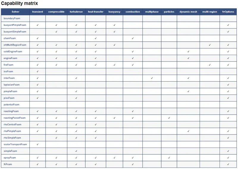
Choosing the Solver
I choose an icoFoam which is used as a Transient solver for incompressible, laminar flow of Newtonian fluids.
Solver capability matrix in OpenFOAM
Results
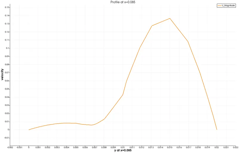
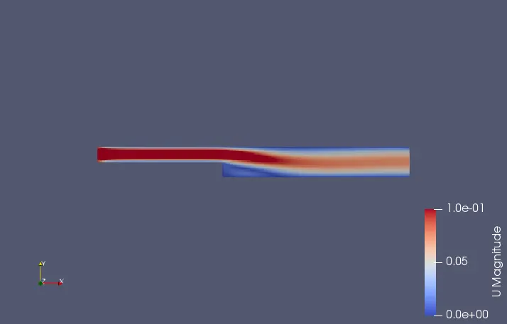
The results show typical characteristics of an incompressible-laminar-viscous flow, that is we see a smooth flow and boundary layer formation as we see that near the step the viscosity remain unchanged because of the boundary layer formation and the flow velocity does not affect the corner area at the step.
Case-1
Case-1 Velocity Profile
Case-1 Velocity profile at x=0.085
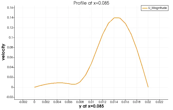
Case-2
The case-2 is exact same as the case one but to capture the boundary layer formation we need a finer mesh near the boundaries this is achieving by using the simple grading option where we decrease the mesh size as at walls and the step.
Case-2 Velocity Profile
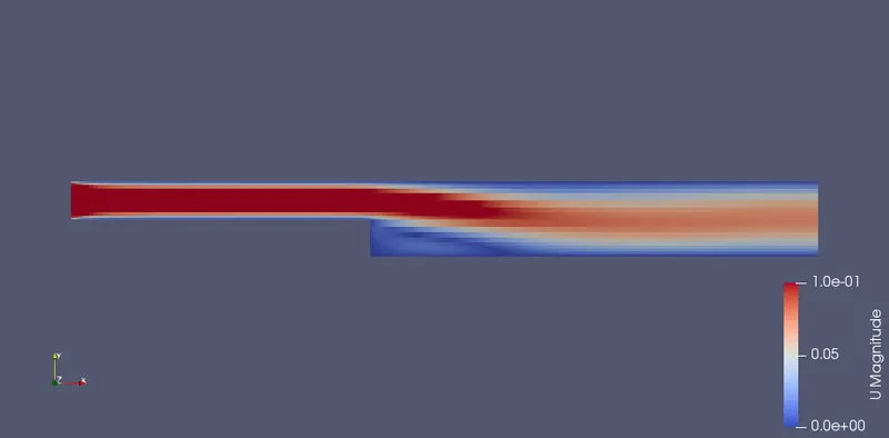
Case-2 Velocity profile at x=0.085