Solving a Second Order ODEs in MATLAB
Solving the second order differential equation to find motion of a simple pendulum with damping
Simple Pendulum
A pendulum is a body suspended from a fixed support so that it swings freely back and forth under the influence of gravity. When a pendulum is displaced sideways from its resting, equilibrium position, it is subject to a restoring force due to gravity that will accelerate it back toward the equilibrium position. When released, the restoring force acting on the pendulum's mass causes it to oscillate about the equilibrium position, swinging it back and forth. The mathematics of pendulums are in general quite complicated. Simplifying assumptions can be made, which in the case of a simple pendulum allow the equations of motion to be solved analytically for small-angle oscillations.
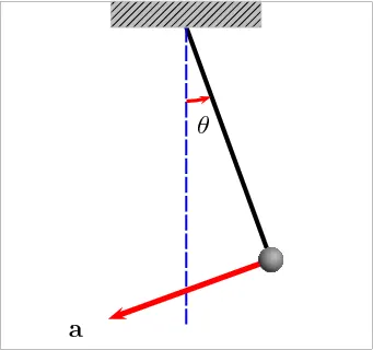
Representation of the motion of a simple pendulum is given by the below equation
`(d^2theta)/dt^2+(gsintheta)/l=0`
where
g = gravity in m/s2,
l= length of the pendulum in m,
`theta=` angle displaced
Considering a damping system is incorporated, the equation of motion of the pendulum becomes
`(d^2theta)/dt^2+b/m (d theta)/ dt+g/lsintheta=0`
where
b=Damping Coefficient
m= mass of the bob in kg
g = gravity in m/s2,
l= length of the pendulum in m,
`theta=` angle displaced in radian
Fomulation of the Program
To find the path we need to solve the second order diferential equation using the ode45 function in Matlab we need to convert the given equation to a first order diferential equation.
`(d^2theta)/dt^2+b/m (d theta)/ dt+g/lsintheta=0`
Let `theta=theta_1` and `(d theta_1)/dt=theta_2` and substituting in the above equation, it becomes
`(d theta_2)/dt+b/m theta_2+g/lsintheta_1=0`
Transforming the above equation
`(d theta_2)/dt=-b/m theta_2-g/lsintheta_1`
To form the above equation we create a function named ode_func where two first order differential equation is store in column matrix (size 2X1)
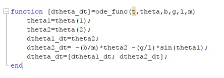
Declaring the given inputs and values.
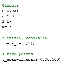
The initial angular displacement=0 and angular velocity=3 rad/sec at t=0 is stored in a column matrix. The first initial condition of angular dispalcment=0 is used to solve the equation to find velocity and the angular velocity=3 rad/sec to solve the equation to find acceleration respectively.
Solving the ODE
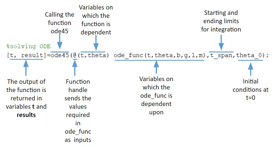
[t,y] = ode45(odefun,tspan,y0), where tspan = [t0 tf], integrates the system of differential equations y′=f(t,y) from t0 to tf with initial conditions y0. Each row in the solution array y corresponds to a value returned in column vector t.
Here 't' is the independent variable upon which the values of function 'y' are dependent. The values of the 'tspan' provided might be occur as same the values in variable 't'.
odefun is the first order differential equation that is to be solved and tspan consists of the limits. The initial conditions at t0 is given in y0.
The ode45 works on the basis of Runge-Kutta method where the limit provided for the integration is discretised into small steps in order to give the required result at any instantaneous time.
The function ode45 takes 3 inputs. The 3 inputs are the function to be integrated, the time span and the initial conditions.
The function would be one like shown in the above example. The time span would be the integration limits. This can be provided as a vector of 2 values, the initial and final time or with a spacing using the linspace function. The solver will choose a step size that is most suitable for the solution to obtain the solution in the most optimal time as possible. The initial condition would be the value of the function at t=0s.
The function can be provided in the form of an anonymous function,
[t,results] = ode45(@(x) x^2, tspan,y0)
Here, we are saying that we don’t know the value of x and that x is an input to the anonymous function that we have defined here. This is equivalent to defining a function that takes the input of x and gives the output of x^2.
The function can also be defined as a separate function. This function must take at least 2 inputs, which should be t and y, apart from other arguments, where t would be the current time and y would be the value of the function at the previous time step.
Assuming we have a function ode, the function must be defined as,
function [output] = ode(t,y,args)
where args refer to any other arguments that the function may take.
This function must then be input to ode45 as
[t,results] = ode45(@(t,y) ode(t,y,args), tspan, y0)
Explanation of the code for solving the ODE
The time interval provided to find the path of the pendulum is discretized in order to get a smooth path for the curve, the input is given to the ode45 solver to find the output for the two differential equation and the result is stored in variable result corresponding to the t.
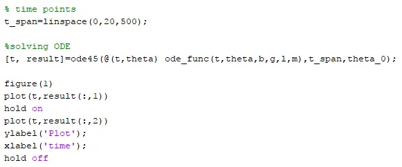
Explanation to get the plot
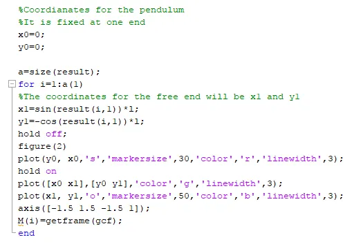
The size of the variable result is used to formulate the for loop according to the number of rows of result.
Here we use only the result corresponding to the equation used to find the displacement as a function of time.
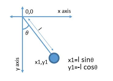
We fix the coordinates of the fixed end of the pendulum at (0,0) and the coordinates of the free end are found using the equation
`x=lsintheta`
`y=-lcostheta`
`-` sign is used with the equation of y because `cos` of `-theta` is positive in 3rd quadrant.
The for loop provides the corresponding values of `theta` and as per the index i. The coordinates are plotted based on the instantaneous values of x1 and y1.
The origin 0,0 is given a square shape with the required size.
The end position (x1,y1) of the pendulum a circle is created with the required size.
The hold on command helps plotting of the succeeding plots and hold off is used at the entry of the for loop to clear the previous plot.
Explanation to record the animation
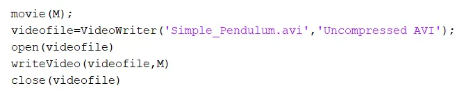
All the instantaneous plots are stored in an array using the getframe. The movie is made by stitching the stored plots. An object videofile is created and using VideoWriter with the required file name and format. Then we open the videofile object and rite the write the the movie in it, at the end we close the object videofile.
Code for solving the path equation and plotiing the results
clear all
close all
clc

%Inputs
b=0.05;
g=9.81;
l=1;
m=1;

% initial condition
theta_0=[0;3];

% time points
t_span=linspace(0,20,500);

%solving ODE
[t, result]=ode45(@(t,theta) ode_func(t,theta,b,g,l,m),t_span,theta_0);

figure(1)
plot(t,result(:,1))
hold on
plot(t,result(:,2))
ylabel('Plot');
xlabel('time');
hold off

%Coordianates for the pendulum
%It is fixed at one end
x0=0;
y0=0;

a=size(result);
for i=1:a(1)
%The coordinates for the free end will be x1 and y1
x1=sin(result(i,1))*l;
y1=-cos(result(i,1))*l;
hold off;
figure(2)
plot(y0, x0,'s','markersize',30,'color','r','linewidth',3);
hold on
plot([x0 x1],[y0 y1],'color','g','linewidth',3);
plot(x1, y1,'o','markersize',50,'color','b','linewidth',3);
axis([-1.5 1.5 -1.5 1]);
M(i)=getframe(gcf);
end

movie(M);
videofile=VideoWriter('Simple_Pendulum.avi','Uncompressed AVI');
open(videofile)
writeVideo(videofile,M)
close(videofile)
The Animation obtained by solving the path equation can be seen at the below link
https://drive.google.com/file/d/1t319Ja5iOI_h-06sTSpoUs1odK5nbKdg/view?usp=sharing
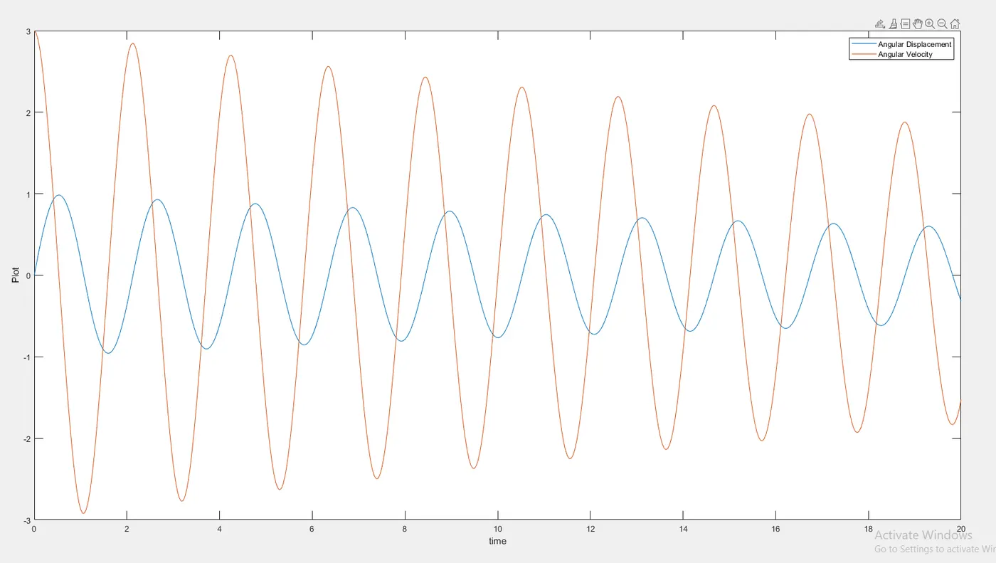
Plot representing Displacement vs Time and Velocity vs Time
Result
It is plot clearly represent the change in displacement and velocity with respect to time at a given damping coefficient. The damping coefficient can be varied in order to get the desired time in which the oscilations must be stopped.