Week 8 - Simulation of a backward facing step in OpenFOAM

Week 8 - Simulation of a backward facing step in OpenFOAM

GIVEN PROBLEM:

• simulate an incompressible-laminar-viscous flow through the backward facing step geometry. You should perform a transient simulation.
• The solver can be chosen based on the described physics of the flow. You need to explain the entire simulation procedure (how you set up the case).
• provide explanations to every change you make inside the reference case files obtained from OpenFOAM tutorials. You can choose the inlet velocity shuch that the flow is laminar.

• perform 2 case studies as described below and compare the results.

  Case 1 - Simulate the flow without using any grading factor (i.e., GF = 1)

  Case 2 - Simulate the flow with grading factor of 0.2. The cells should be finer near the walls (includig the step wall).

• You can use the following mesh parameters but you can feel free to modify these values.

  Mesh specification

  1. Number of cells along the x direction (longer dimension) = 200
  2. Number of cells along the longer y direction = 20;

• Boundary condition specification

  The domain specifications are provided in the following figure.

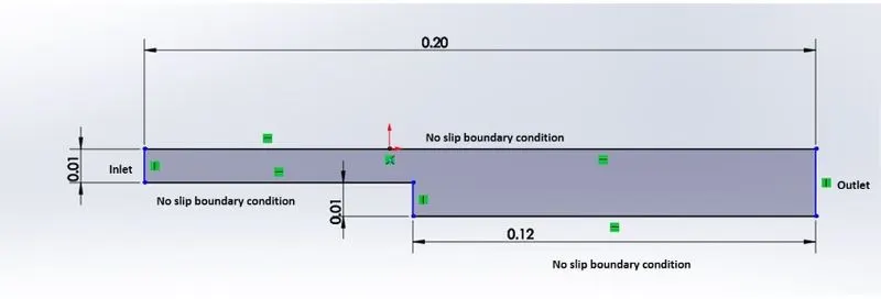
Desired output

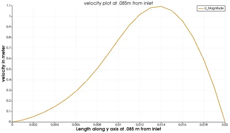
• Measure the velocity profile at 0.085 m from the inlet of the geometry for both case studies and compare. You can use the plot over line tool for this.
• Explain why Grading/Growth factor is essential for meshing.

THEORY AND PERFORM:

In order to start we have to open terminal in linux operating system by pressing alt+ctrl+T and then we have to follow below operations:

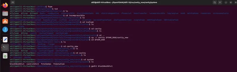
1. First of all we are going to solve the problem using openFoam and we have to use tutorial in openFoam.so we type foam in the terminal and then tut to open the tutorial .

2. We have to solve incompressible problem in the simulation so after typing 'ls' to know the list of directory type cd incompressible to open the directory.Then type ls , we can see the solvers in the folder.

3.icoFoam is the solver that is used to solve laminar transient of newtonian flow so we type cd icoFoam next.Then typing ls we can explore the folder.Here we get cavity folder which is used to create the required blockmesh.

4.In cavity again we are going to get cavity folder where we are going to create our required mesh.so we type cd .. to come out of the cavity folder and then type cp -r $FOAM_RUN/cavity_new to copy the cavity folder in the $FOAM_RUN folder and give it a new name cavity_new .

5. Then we open the $FOAM_RUN folder by typing cd $FOAM_RUN , then by ls open the folders within it , the type cd cavity_new to open the folder and then ls to open the cavity_new folder . Then ls to know the folders inside it.

6. Inside the cavity_new folder we get the system folder by typing cd system , the ls to open folders inside it ,then we get the blockMeshDict file . so we open the file by gedit blockMeshDict.

WHAT IS blockMeshDict FILE?

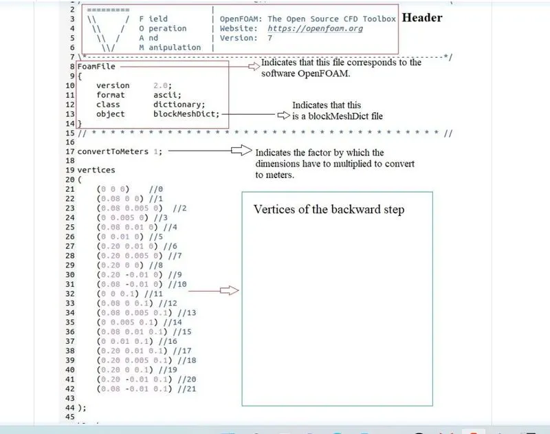
When we open the 'blockMeshDict' file we are going to see the following script file. First we can see the Header option which is a comment section not exeutable.Then we get the Foamfile section which says the information about the script file in two sectiions - keys and values . One value in it blockMeshDict of object key. Then we are getting convertToMeter section where we are going to change the all lengths into meter.Then we are getting vertices section where we are getting the points that we have to use to create the figure,there we are getting the box portion where we are getting the hex section to specify the position of the blocks to create the overall figure.

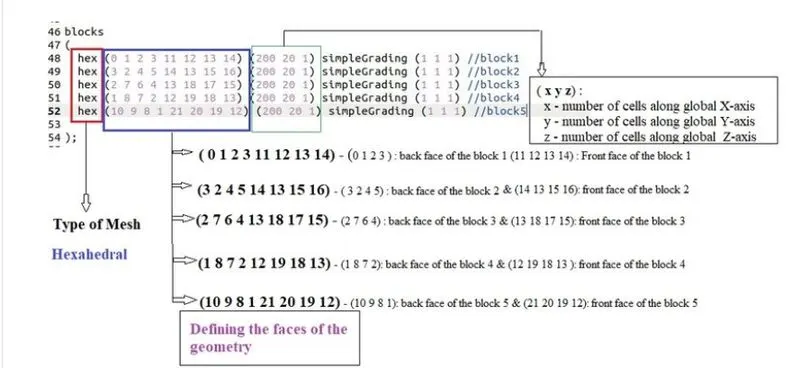
Above we have seen how to choose the hex portion, then we are going to see about boundary portion below.

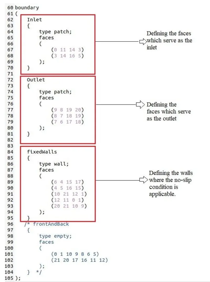
EDITING THE blockMeshDict file:(Mesh generation without the grading factor)

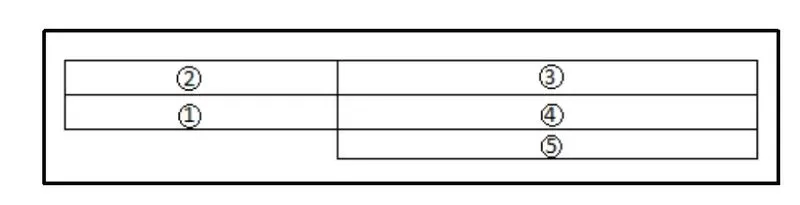
First of all we have to choose the vertices by (x,y,z) coordinates starting from (0,0,0) . so we have to create the following geometry.

To create the geometry let us consider the geometry as 5 blocks following below

Now we are providing vertices of each block by providing the following sketch

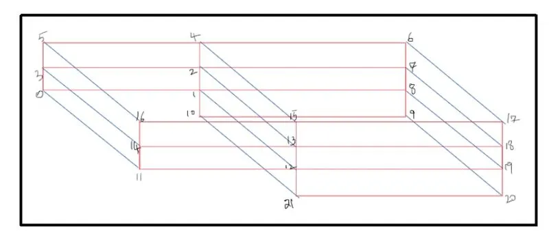
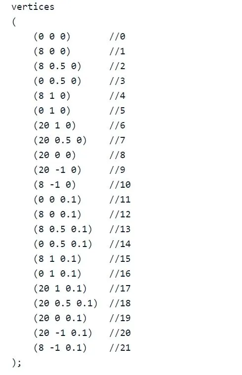
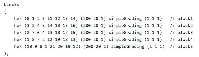
Next we are going to define blocks for meshing .If we look at the mesh format first letter , in the block paranthesis is hex which define type of mesh which is hexahedral mesh. Then again in paranthesis we provide the vertices number according to order which follow the right hand thumb rule, thumb in the z axis and order of fingers follow rotational order.Then comes number of mesh grid which we want to divide along x,y and z length.we define it as(nx,ny,nz)format.

GIVEN MESH SPECIFICATION:

1. Number of cells along x direction =200

2.Number of cells along y direction= 20

Lastly we give simple grading which is expansion ratio among cells.

Grading factors or expansion ratios:

The expansion ratio enables the mesh to be graded or redifened in specific direction.The ratio that of the width of the one end cell along the one end of a block to the width of the start cell along the edge as shown in the figure:

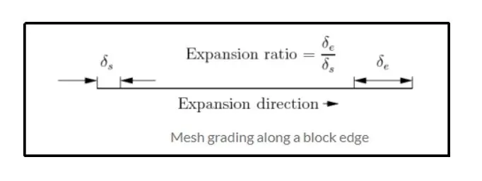
In simple format EXPANSION RATIO=(size of end cell/size of start cell)

Here simplegrading (1,1,1) so expansion of the blocks are uniform in all direction.We have 5 blocks to define hex mesh of 5 blocks.

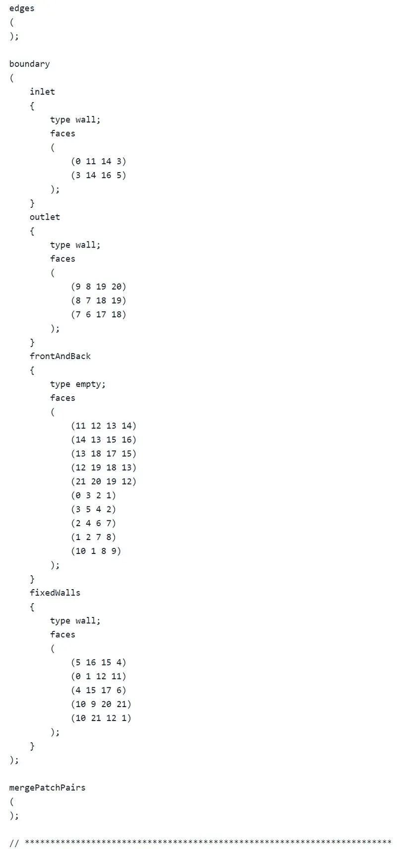
NEXT we are going to define boundary conditions:

After editing the blockMeshDict file save it (ctrl+s) and close it.

Next step is to navigate to controlDict file.

WHAT IS controlDict file?

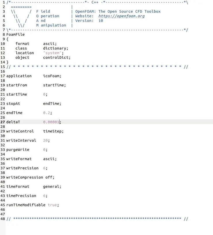
controlDict file provides the time limit - start time and end time , also it specifise deltat.while selecting deltat CFL value should be less tjan one .Otherwise solution would stop forcebily and it may diverge at the time of converging .

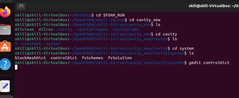
By following above process in the terminal window we open the controlDict file.

EDITING controlDict file by the following way

WHAT IS VELOCIY AND PRESSURE FILE?

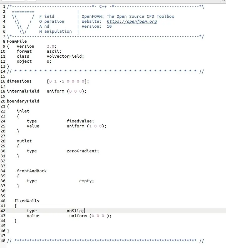
We have to set the initial condition of pressure and velocity at each faces and also keep the name of the boundaries same as we change in blockMeshDict file.

VELOCITY FILE:

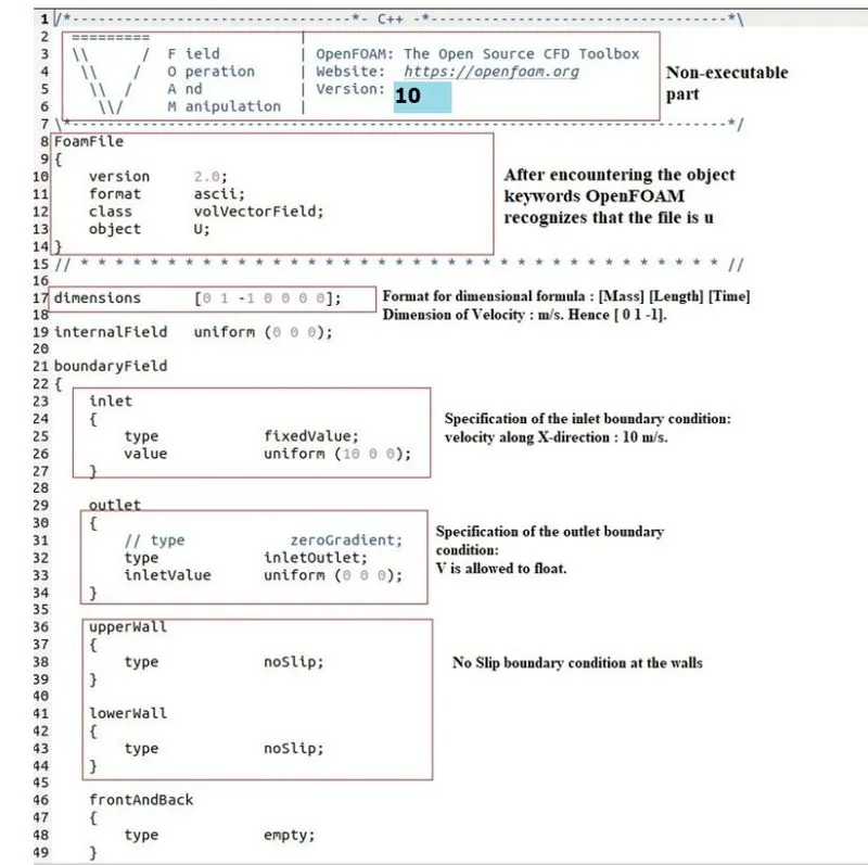
EDIT VELOCITY FILE:

PRESSURE FILE:

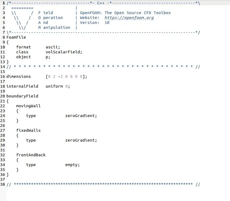
EDIT PRESSURE FILE:

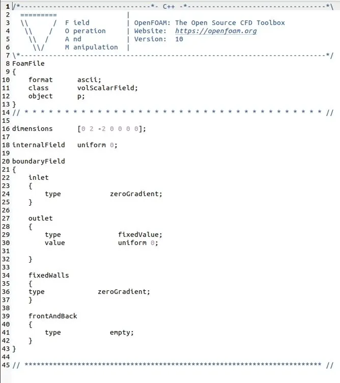
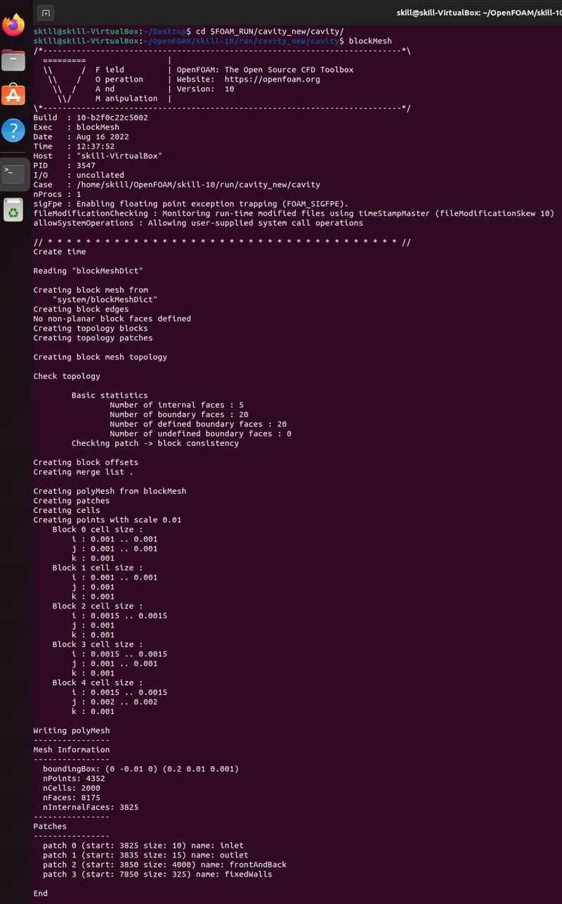
At this point our problem statement is set and we can now proceed to deploy mesh using blockMesh command and then checkMesh command to check if there is any error in our mesh.

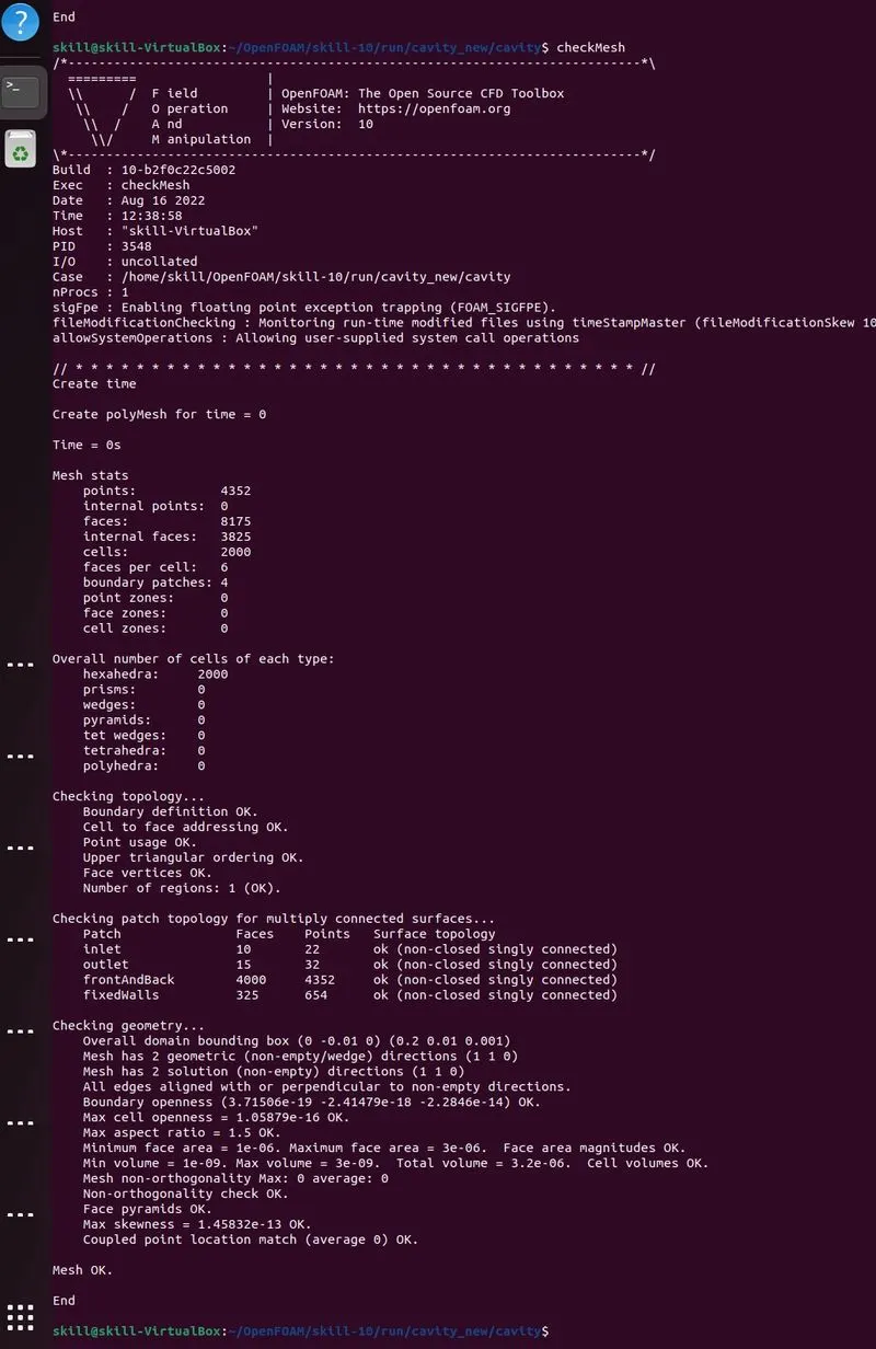
Now we have checked that is our mesh is as per our requirement and to view we type paraFoam command next.

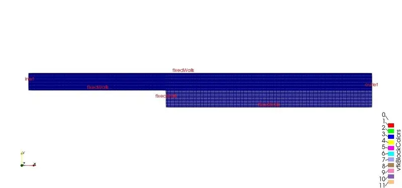
From the above mesh we can see that it is not uniform all over . so let us adjust the meshgrid in the following way

After making the above changes

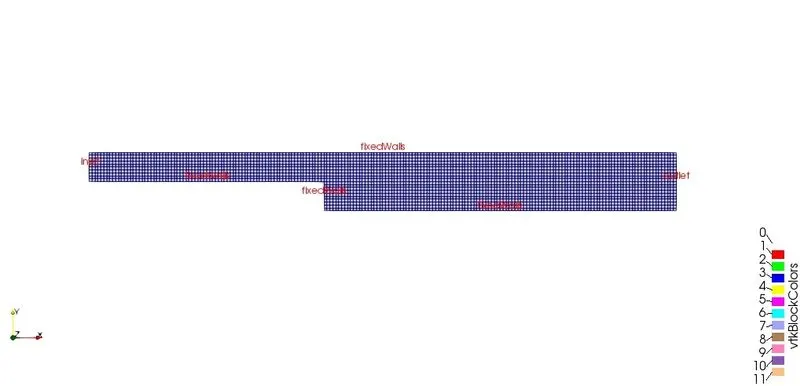
Now the mesh is uniformly distributed.

Now we type icoFoam command because simulation that was selected was icoFoam.

Result:

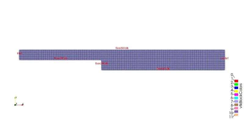
mesh grid:

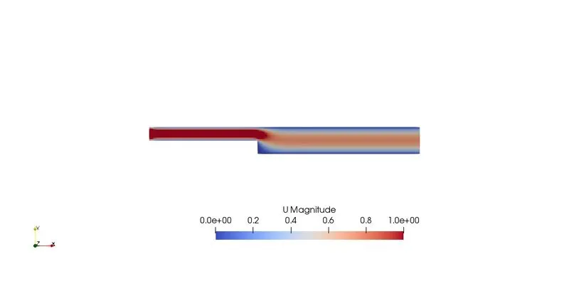
velocity Distribution along the domain area:

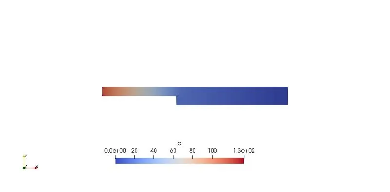
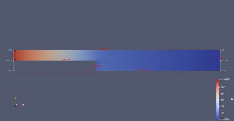
Pressure Distribution along the domain area

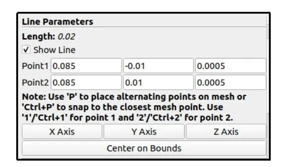
To calculate velocity at 0.085m from inlet modify the following parameters:

velocity plot:

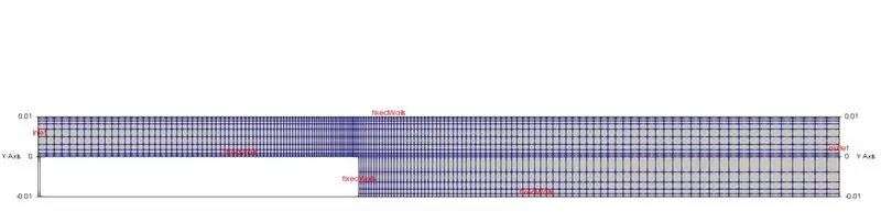
WITH GRADING FACTOR 0.2(CELL NEAR FIXED WALL):

blocks

{

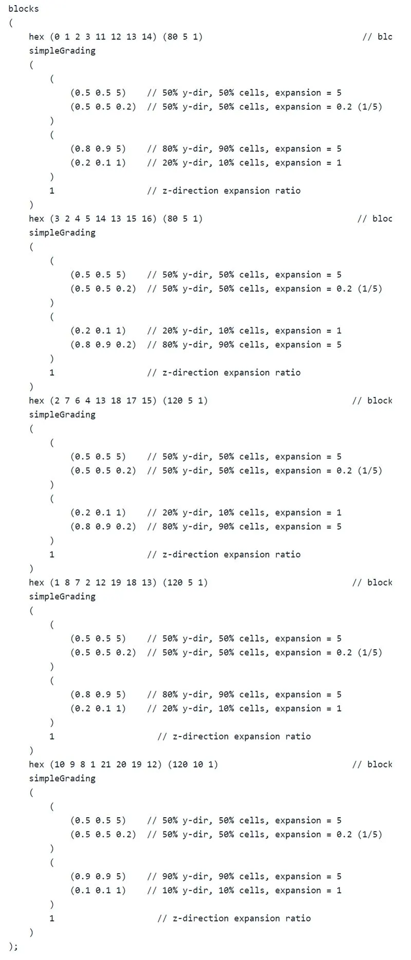
hex(0 1 2 3 11 12 13 14) (80 5 1) simplegrading(0.2 5 1) // block1 (1/0.2)=5

hex(3 2 4 5 14 13 15 16) (80 5 1) simplegrading(0.2 0.2 1) //block2

hex(2 7 6 4 13 18 17 15) (120 5 1) simplegrading(5 0.2 1) // block3 (1/0.2)=5

hex(1 8 7 2 12 19 18 13) (120 5 1) simplegrading(5 5 1) // block4 (1/0.2)=5

hex(10 9 8 1 21 20 19 12) (120 5 1) simplegrading(5 5 1) // block5 (1/0.2)=5

};

output mesh for above code:

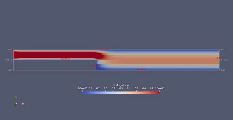
velocity Distribution along the domain area:

pressure Distribution along domain area:

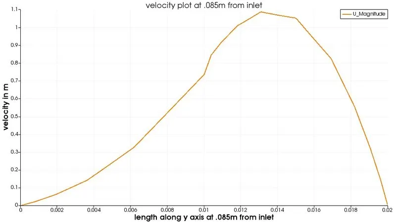
velocity plot:

With grading factor 0.2 (cell near all walls):

Next using grading factor 0.2 in following way

output mesh for above code:

velocity Distribution along the domain area:

pressure Distribution along domain area:

velocity plot:

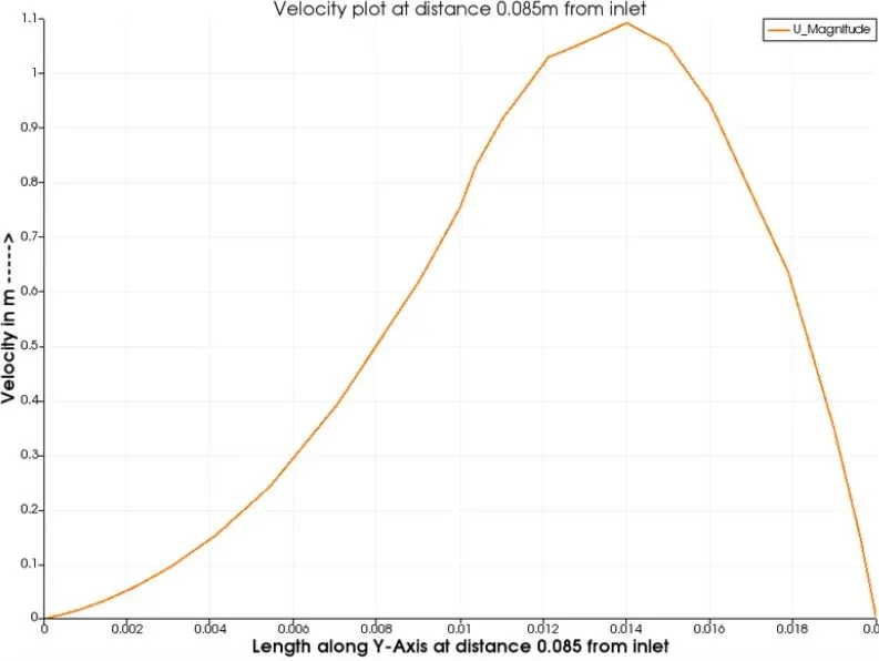
RESULT:

upto this point we have plotted velocity plot for both without grading factor and with 0.2 grading factor cases . If we take a look at all three line graph we can see the plot for velocity without grading factor seems more smooth and accurate than other two plot.so one can say grading can distrupt out result , but it is incorrect. Because if we take a good look at it we can notice the mesh is fine at step wall along x axis and course along y axis.so we are not getting smooth plot for velocity at .085 m from y axis .

- To understand this thing clearly we can see below figure where we can see on the left side there is a coarse mesh and on the right side fine mesh .Above picture there respective graphs are presented , whichcan really convince anyone how at any given point the produce a plot.The one on the right side mesh there is a very smooth plot except one small pick at point .01 and on the other hand for coarse structure mesh the curve of graph and curve is not smooth , there are sharp corner forming at the top of the graph.

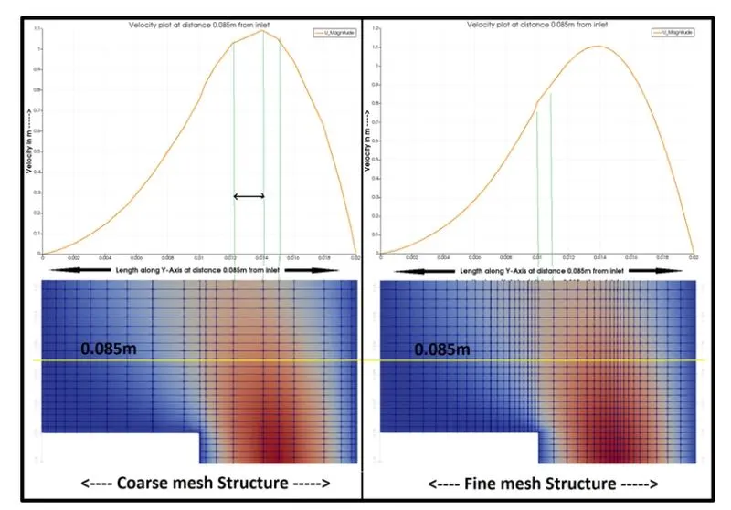
AFter learning how mesh actually works we should use fine mesh near the point where we can expect our results. In CFD fluid always shows large changes near the wall and obstucles along its way and to capture those changes effectively we always use grading or finer mesh near the wall.

-To get effective and relible result one should know finer grading factor .In a bid to obtain more effective result,suppose,we use large number of fine elements it could use large computational time and use large computational memory(RAM).So that use of grading is important so that we can use fine mesh to capture the flow at boundary walls and obstacles ,course mesh at more open area .

- We can also see the importance of fiem mesh by observing following picture .as grading factor increases near step, the resoltion of image is improving .Means as the number of elements increasing the flow result also increasing .

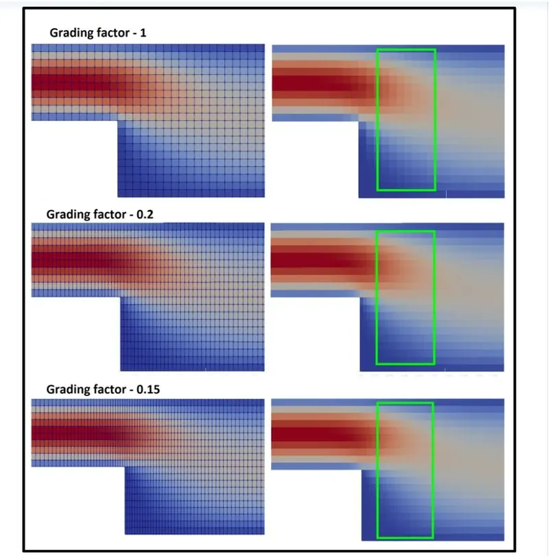
-We can see more fine result at grading facotr 0.15. Hence always use fine mesh inthe area where maximum changes happen in velocity, pressure or other property of fluid to capture more detail and accurate result.