Week 8 - Simulation of a backward facing step in OpenFOAM
AIM:
The objective of the report is perform a simulation of incompressible-laminar-viscous flow through the backward facing step geometry and validate the results.
PROBLEM STATEMENT:
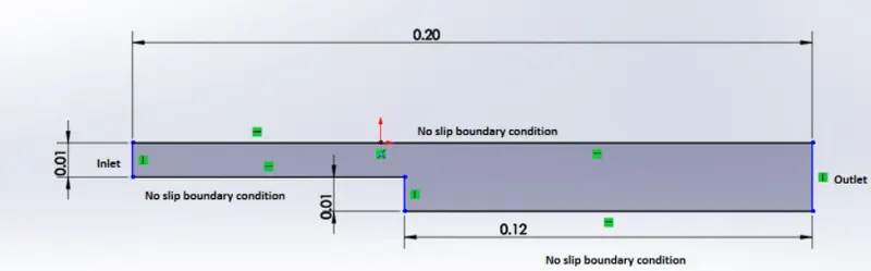
Given,
Backward facing step geometry of dimensions -
INLET = 0.01 m
OUTLET = 0.02 m
LENGTH = 0.2 m
FLOW TYPE - Incompressible laminar viscous flow
SOFTWARE - Open foam
Open Foam is a open source software. It is not a slover but a C++ tool box with a range of solvers, pre and post processing utilities.
PROCEDURE:
In CFD, along with the Navier-Stokes equation, different physical models are represented by different types of equations. So, different numerical schemes are used to obtain a stable solution. In Open Foam, different physical models are solved by using different solvers.
For Incompressible-laminar-viscous flow, ICO FOAM solver is used.
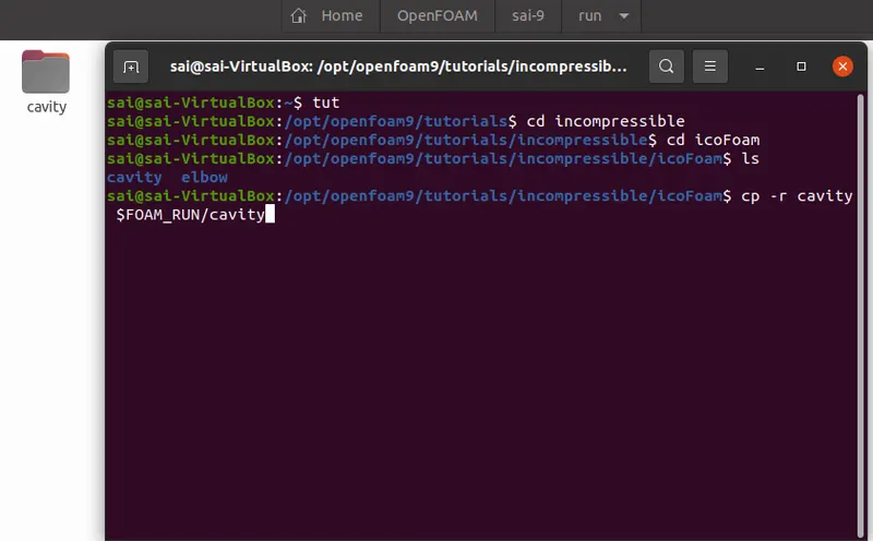
In this report, instead of simulating the model from scratch, we considered ICOFOAM -> CAVITY model as reference and changes are made to this model as per the problem statement. So, Initially copy the Ico foam -> cavity folder present in the tutorial folder to run folder in ubuntu by this command.
Steps in CFD - Preprocessing, Solving and Postprocessing
1)Pre-processing -
Pre-processing is an initial step in CFD, where the domain is discretized into a finite number of cells and boundary conditions are applied.
In Open Foam, there are two ways of creating a mesh - a) Importing the mesh, that was generated in other software tools. b) Creating the mesh in Open Foam itself by using BLOCK MESH (or) SNAPPY HEXA MESH.
In this report, the mesh is generated by using block mesh. So, edit the blockMeshDict file present in the system folder as per the problem statement.
Geometry Creation -
The domain is discretized into five blocks as shown in the figure.

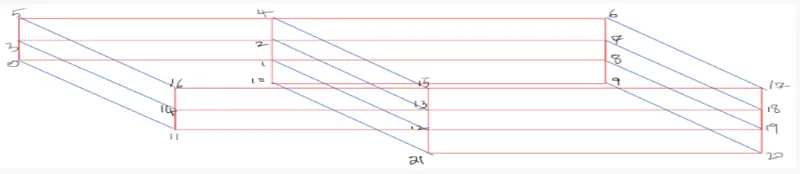
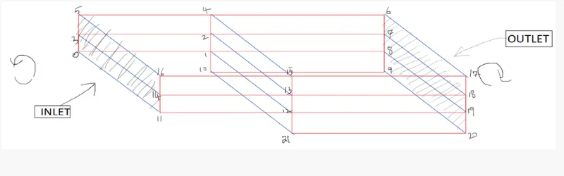
In this report, 2 different mesh patterns are generated and the results are validated.
Mesh generation -
- Number of cells along the x direction (longer dimension) = 200
- Number of cells along the longer y direction = 20;
Case (a) - Mesh size is uniform throughout the domain
The blockmeshdict file for the given problem statement is edited as shown in fig.
NOTE - MKS unit system is followed.
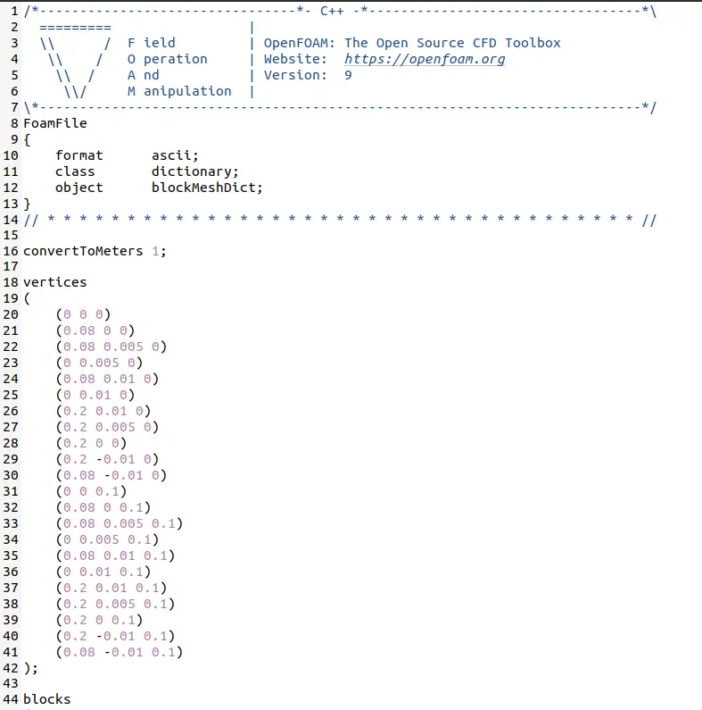
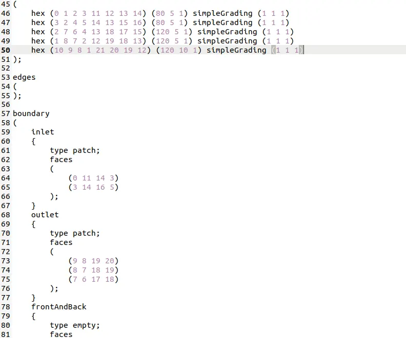
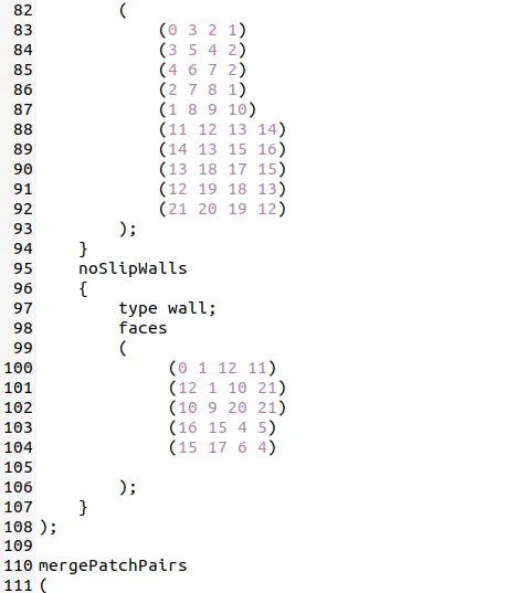
The vertices line indicates the coordinates of corner points of each block.
The block line indicates the vertices associated with each block and no.of cells present in each block. Simple grading(1,1,1) indicates uniform mesh flow in the block.
Boundary line indicates the boundary types associated in the model.
Since, we are considering 2D flow and it is represented in Open Foam by 1 cell in z - direction with a cell size of 0.1m in z -direction.
The blockMesh command in terminal generates mesh, which is stored in the CONSTANT -> POLY MESH folder.
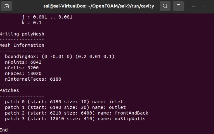
checkMesh command in the terminal checks whether the mesh is successfully created or not as shown in the fig. At the end, mesh ok indicates mesh is generated succesfully.
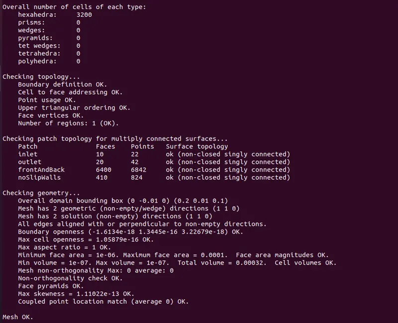
Case (b) - Mesh size with grading factor of 0.2 is generated with finer mesh near the walls of uniform mesh flow.
Grading factor = size of end cell / size of start cell
The blockmeshdict file for the given problem statement is edited as shown in fig.
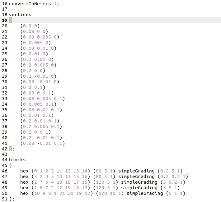
Simple grading (0.2 5 1) indicates, grading factor of 0.2 in x-direction, grading factor of 5 in y-direction and grading factor of 1 in z-direction.
Fluid Properties -
The kinematic viscosity = 0.01 m2/s
Boundary Conditions -
The pressure and velocity field variables are calculated in this model.
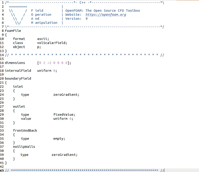
At Inlet - P = zero gradient
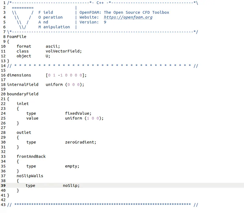
V = 1 m/s
At Outlet - P = zero gauge pressure
V = zero gradient
At Walls - P = zero gradient
V = no slip condition
The boundary conditions are present in the '0' folder and the following fig shows the Pressure and velocity boundary condition file.
Termination -
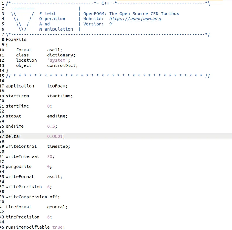
The control termination file is present in the 'system' folder as shown in the fig.
The simulation time is set for 0.5sec, dt = 0.0001sec
2)Solver -
For Incompressible-laminar-viscous flow, ICO FOAM solver is used.
Case (a) - IcoFoam command in the terminal window executes the simulation for uniform mesh as shown in the fig.
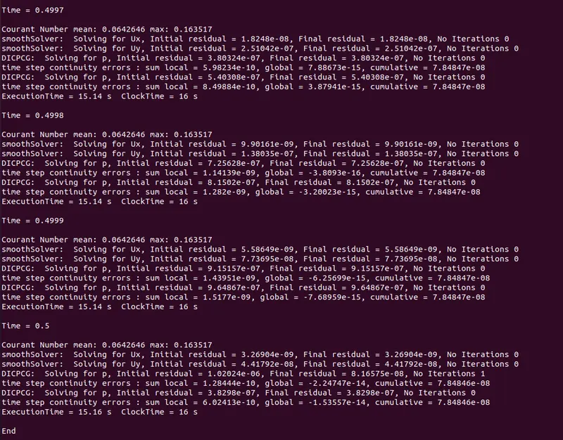
The total execution time is 15.16 sec, Clock time is 16 sec. The max Courant number considered in this simulation is 0.163 which is feasible.
Case (b) - IcoFoam command in the terminal window executes the simulation for non-uniform mesh as shown in the fig.
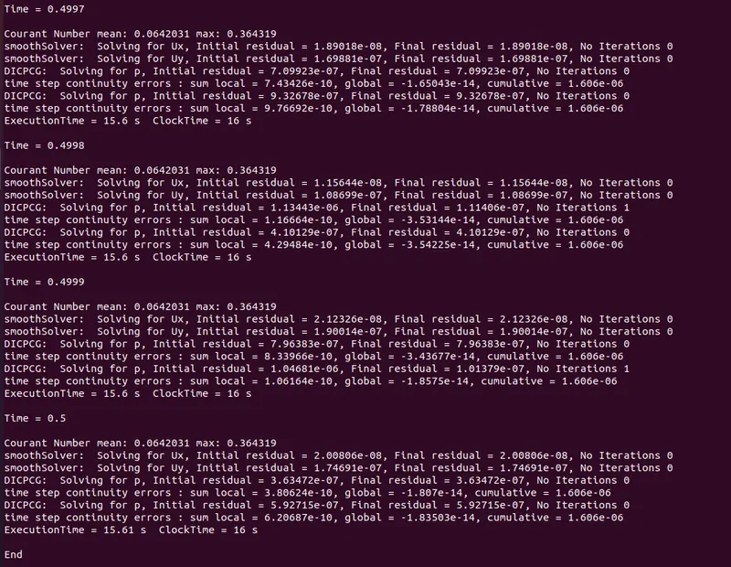
The total execution time is 15.61 sec, Clock time is 16 sec. The max Courant number considered in this simulation is 0.364 which is feasible.
3)Post-processing -
In openFoam, inorder to view the results ParaView tool is used. To activate paraview, type paraFoam command in the terminal window. The following fig shows the uniform mesh and non-uniform mesh results.

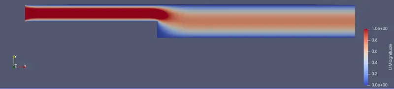
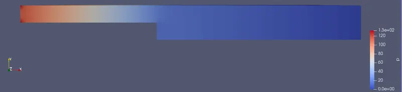
FIG 1- Uniform mesh flow
In fig 1, the middle fig represents the velocity flow field in the domain. At inlet, the velocity is around 1m/s and at the walls, blue contour indicates zero velocity as no-slip boundary condition is given.
In Pressure contour, the max gauge pressure is at inlet of value 130 Pa/(kg/m3) and minimum gauge pressure is zero which indicates the pressure value is atmospheric pressure.


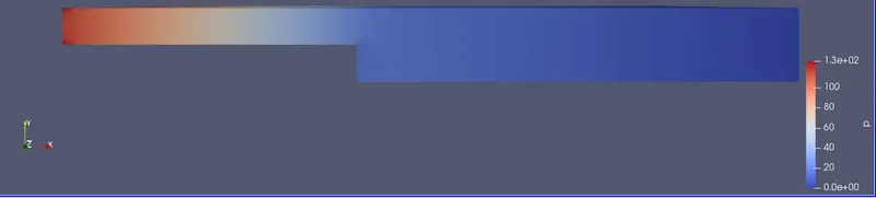
FIG 2- Non uniform mesh with finer mesh at the boundaries and step region
In non-unform mesh, the mesh is finer at the walls and step region compared to uniform mesh. So, accurate results are obtained in the non-uniform mesh compared to uniform mesh. In macroscopic view, we cant clearly able to distinguish the results in Fig 1 and Fig 2. By increasing the magnification factor, we can distinguish the results as shown in fig 3.
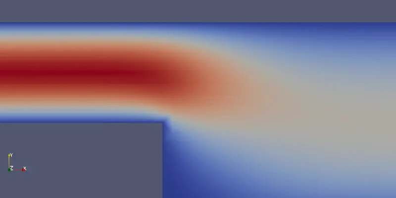
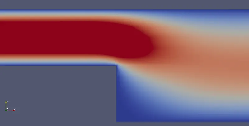
FIG 3 - Uniform mesh v/s Non uniform mesh
In fig 3, the left image is velocity profile in uniform mesh and the right part is velocity profile in non-uniform mesh. It is clearly observed that finer mesh produces accurate results compared to coarse mesh.
In fig 4,5 the x-axis indicates the points inside the domain at section 0.085 m from the inlet. As in model, the dimension at section is 0.02 m, so in plot, the x-axis ranges from 0 to 0.02. In plot, x = 0 indicates the bottom face and x = 0.02 indicates the top face.
In the model, since the flow is laminar, at fully developed region parabolic velocity profile is obtained as shown in fig 4,5.
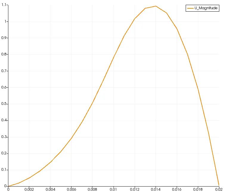
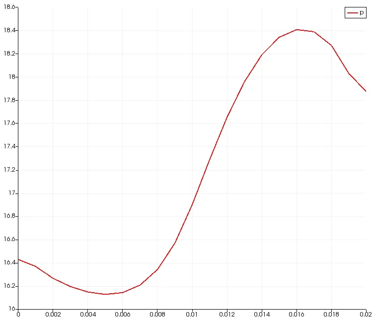
FIG 4 - Velocity and Pressure at section x=0.085m for uniform mesh
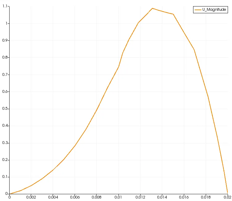
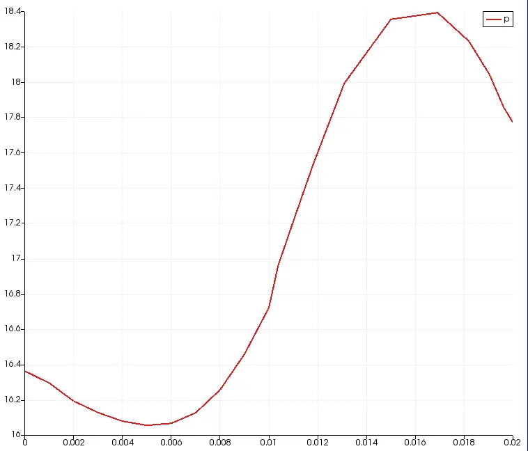
FIG 5 - Velocity and Pressure at section x=0.085m for non-uniform mesh
In fig4, in the velocity profile it is observed that the max velocity occurs at x=0.014m and in fig5 velocity profile, the max velocity occurs in the region between x = 0.012 and x = 0.014.
From fig 4,5 it is clearly observed that in uniform mesh the curves in the plots are smooth compared to the curves in the plots of non-uniform mesh. As in uniform mesh since the mesh is coarse the results are approximated by some approximations which results in the smooth curves. In non-uniform mesh, since the mesh is fine at the step region, more accurate results are plotted compared to uniform mesh which results in sharp curve lines.
In plots,For coarse mesh at x = 0.013, velocity(u) = 1.079m/s , pressure(P) = 17.9583 Pa/(kg/m3)
For Fine meshat x = 0.013, velocity(u) = 1.082m/s , pressure(P) = 17.9614 Pa/(kg/m3)
Percentage error in velocity is 0.27% and in pressure is 0.0176%.
CONCLUSION:
At flow changing areas, it is recommended to use fine mesh. Since, the fine mesh produces accurate results compared to coarse mesh. But the computational time to simulate fine mesh is more compared to coarse mesh.