Simulating Cyclone separator with Discrete Phase Modelling
Simulation Procedure :
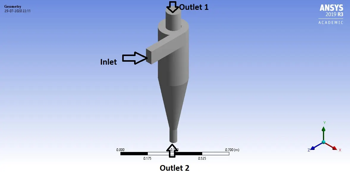
Geometry
- Import the geometry.
- Extract the fluid volume & check for any extra edges so the fluid volume don't get obstruct.
- Suppress the outer geometry.
- This completes the geometry section.
Mesh
- Open the mesh section
- Name the faces like inlet, outlet-1,outlet-2.
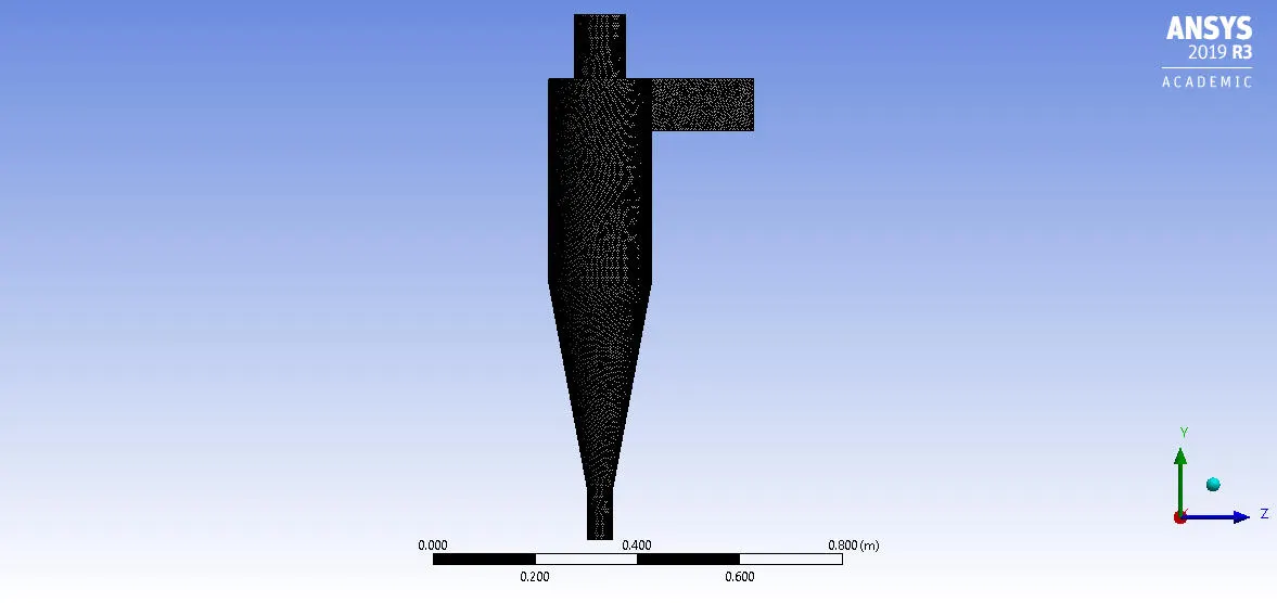
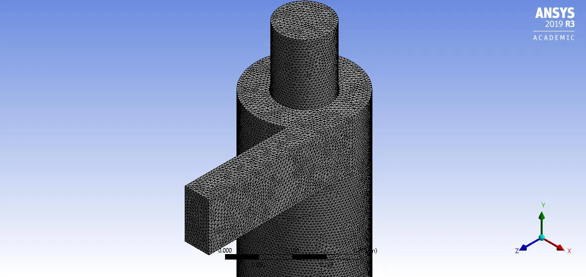
- Then generate the mesh(in our case we have used 0.0055 m mesh element size).
Setup :
- Perform mesh check
- Set up gravity
- Turn on the Turbulence model, In our case we are using K-epsilon RNG model as it is good for swirl domination flows.
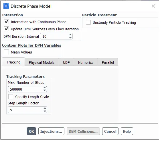
- Set up the DPM and DPM iteration interval.
- Then add injections to inlet surface and set up point properties like particle velocity, Diameter and flow rate.
- Set the boundary conditions.
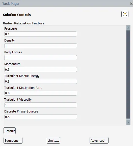
- Set up the solution method and relaxation factors.
- Finally initialize and run the setup.
- Export the particle history.
Result :
- Make the fluid volume visible.
- Import the particle data.
- Set the particle tracks and color them with required variables.
- Set up quick animation and observe the particle flow.
Mesh Input :
1] Element size = 0.0055 m/5.5 mm
2] Total elements = 459278
Setup Inputs :-
1] Solver - Pressure Based Steady
2] Viscous Model - K-epsilon RNG(Swirl Domination Flow)
3] Particles - Anthracite
4] Fluid - air
5] DPM Boundaries - Inlet = Reflect
Outlet 1 = Escape
Outlet 2 = Trap
6] Solution method - SIMPLE(first order)
7] No. of DPM tracking steps - 50000
Outputs
########################## { CASE I : Simulation on Varrying particle Diameter } ##########################
In this case we are going to vary particle diameter from 1μm - 5μm and keep the particle and flow velocity as 3m/s and calculate the separation efficiency for each case.
<<<<<<<<<<<<<<< [ For Particle Dia. = 1 μm] >>>>>>>>>>>>>>>
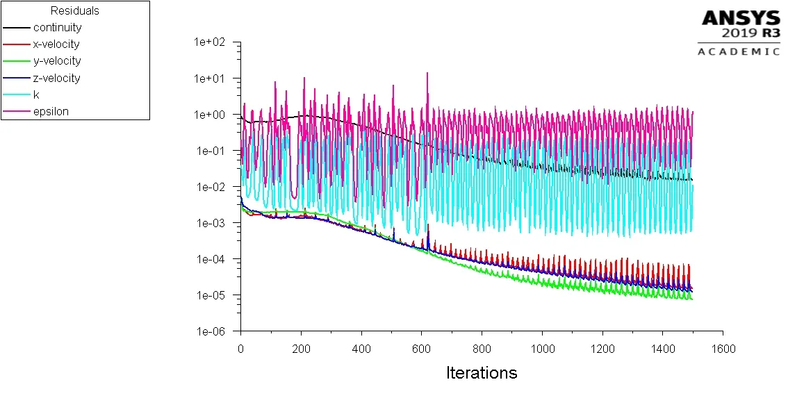
- Residual
- Particle time
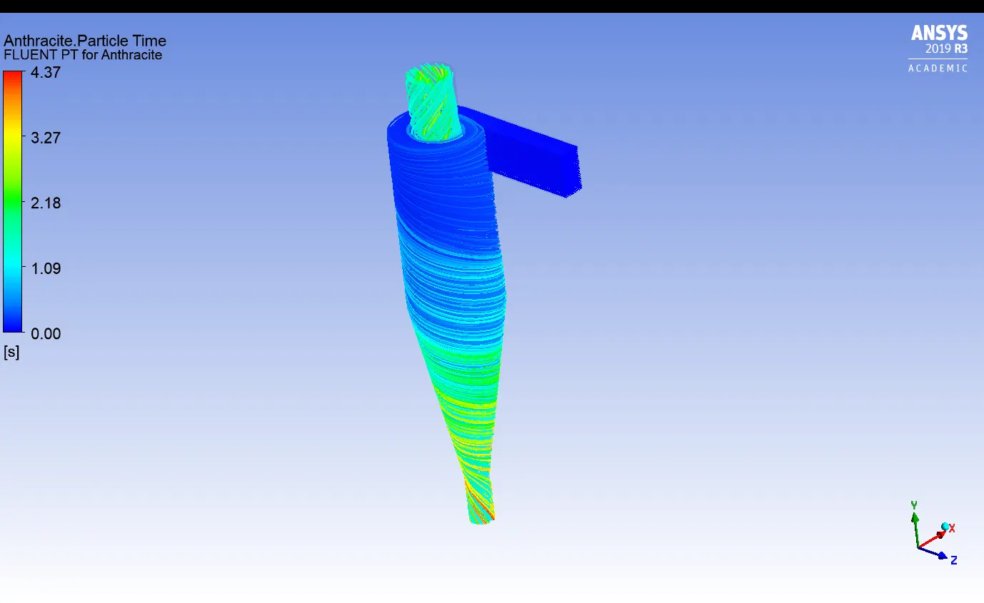
- Particle animation
Particle Info. :
| Tracked | Escaped | Trapped | Incomplete |
| 350 | 159 | 189 | 2 |
<<<<<<<<<<<<<<< [ For Particle Dia. = 2 μm] >>>>>>>>>>>>>>>
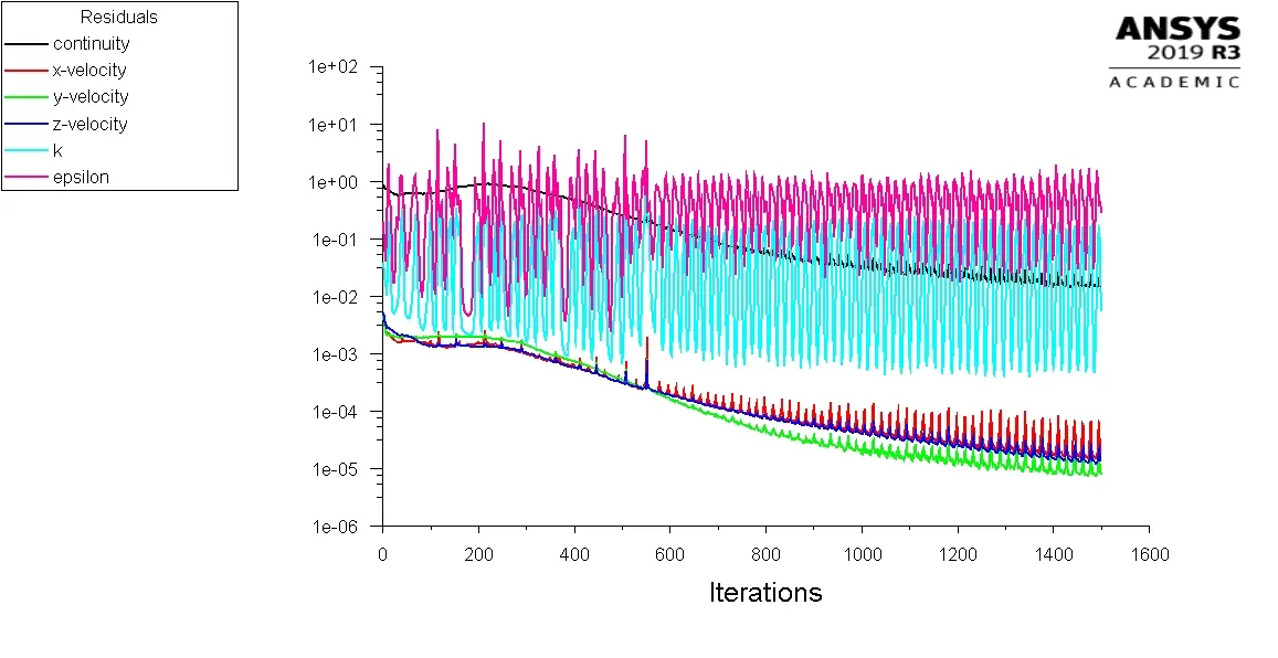
- Residual
- Particle time
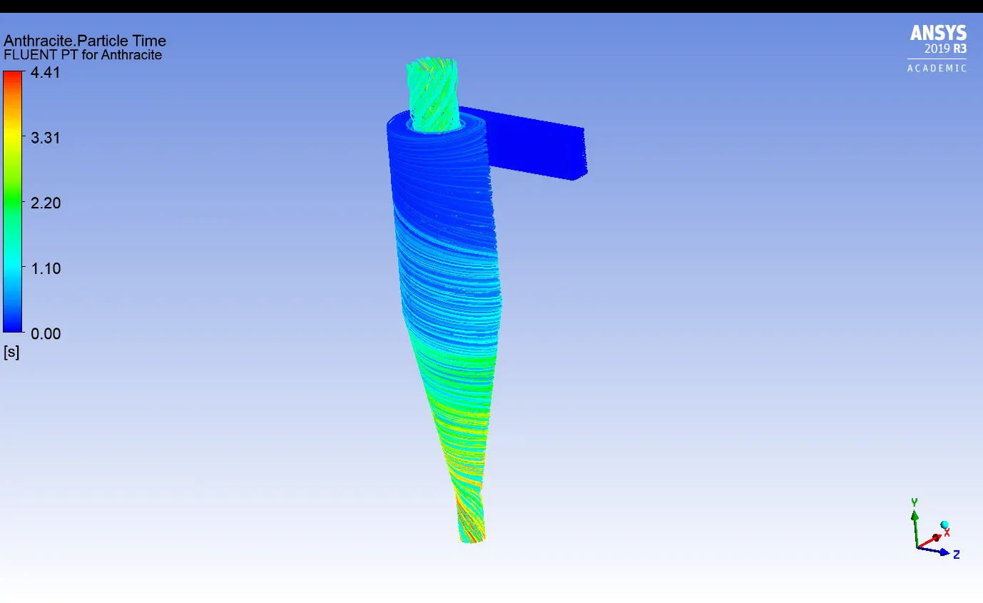
- Particle Animation
Particle Info. :
| Tracked | Escaped | Trapped | Incomplete |
| 350 | 141 | 207 | 2 |
<<<<<<<<<<<<<<< [ For Particle Dia. = 3 μm] >>>>>>>>>>>>>>>
- Particle time
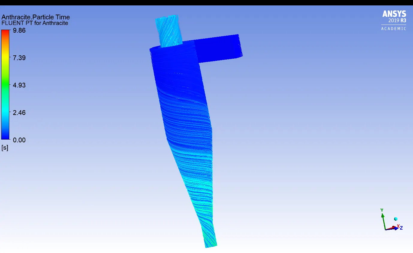
- Particle animation
Particle Info. :
| Tracked | Escaped | Trapped | Incomplete |
| 350 | 124 | 225 | 1 |
<<<<<<<<<<<<<<< [ For Particle Dia. = 4 μm] >>>>>>>>>>>>>>>
- Residual
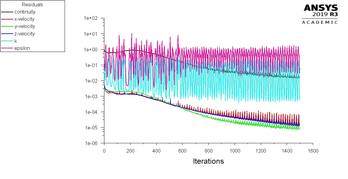
- Particle Time
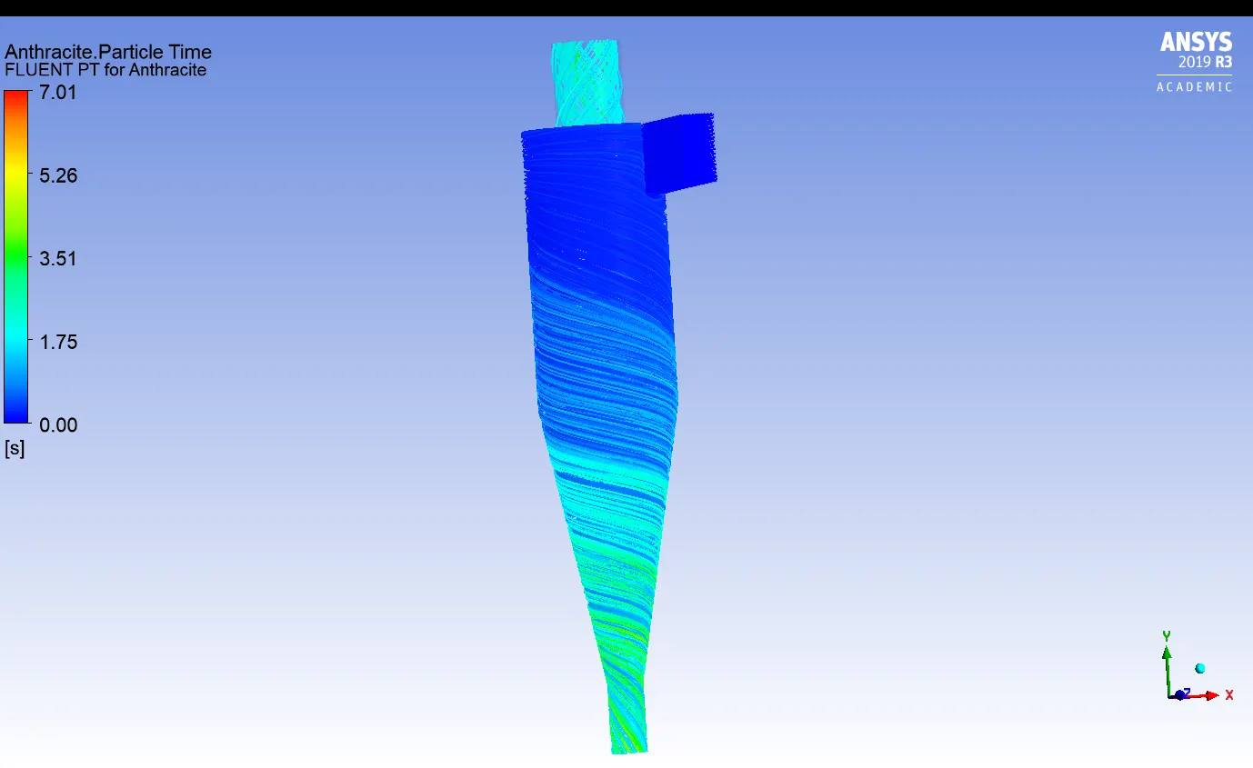
- Particle Animation
Particle Info. :
| Tracked | Escaped | Trapped | Incomplete |
| 350 | 102 | 245 | 3 |
<<<<<<<<<<<<<<< [ For Particle Dia. = 5 μm] >>>>>>>>>>>>>>>
- Residual
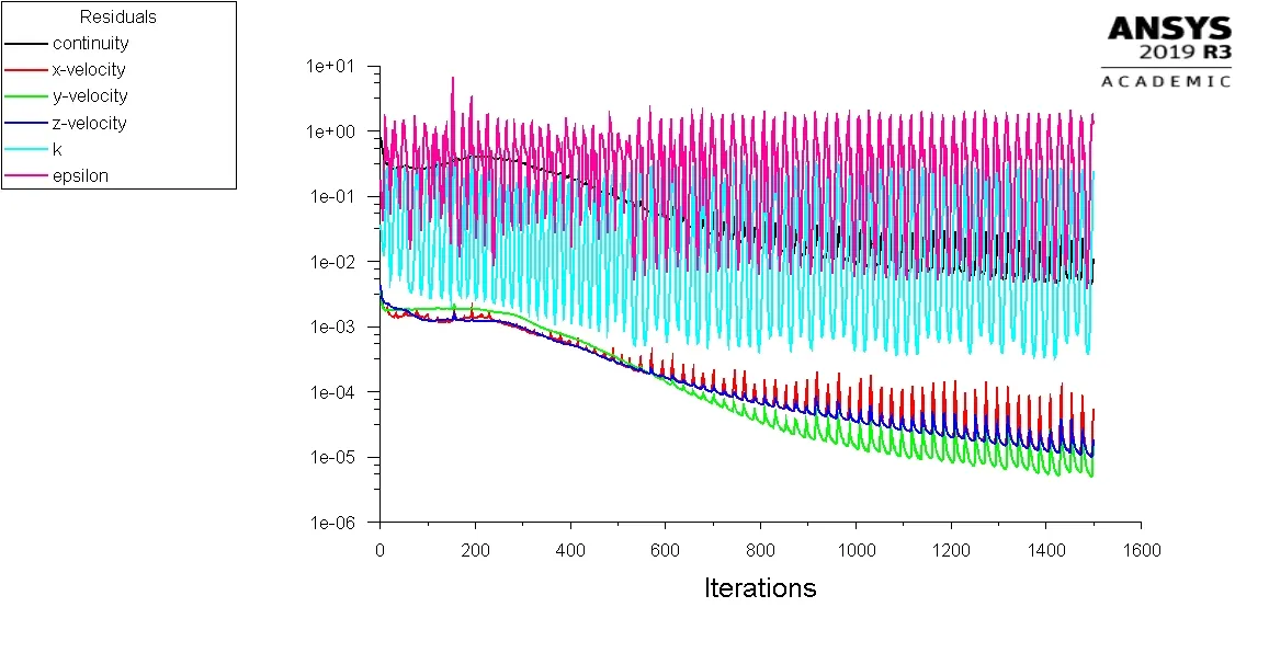
- Particle animation
Particle Info. :
| Tracked | Escaped | Trapped | Incomplete |
| 350 | 68 | 278 | 2 |
Seperation Efficiency = (Particles Trapped/Particles Tracked) * 100
| Particle Dia. | Trapped | Tracked | Efficiency |
| 1μm | 189 | 350 | 54% |
| 2μm | 207 | 350 | 59.14% |
| 3μm | 225 | 350 | 64.28% |
| 4μm | 245 | 350 | 70% |
| 5μm | 278 | 350 | 79.42% |
########################## { CASE II : Simulation on Varrying particle and flow Velocities } ##########################
In this case we are going to vary particle and flow velocity from 1m/s - 5m/s and keep the particle diameter as 5μm and calculate the separation efficiency & pressure drop for each case.
<<<<<<<<<<<<<<< [ For Velocity : 1m/s ] >>>>>>>>>>>>>>>
- Specifically for this case only with velo. 1m/s, we are going to use different mesh settings and higher number of DPM tracking steps(500000), as the velocity is too low and also the Max. elements restrictions, it is difficult to capture particles which ultimately results in higher incomplete particles, as the no. of mesh elements(0.5 million) aren't enough with this case with lower velocity.
- Also we need to relax the pressure & momentum equation to get better results.
mesh element size - 0.00531 m/5.31 mm
total elements - 495457
DPM setting-
Under -relaxation factor -
Outputs -
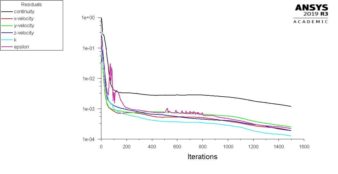
- Residual
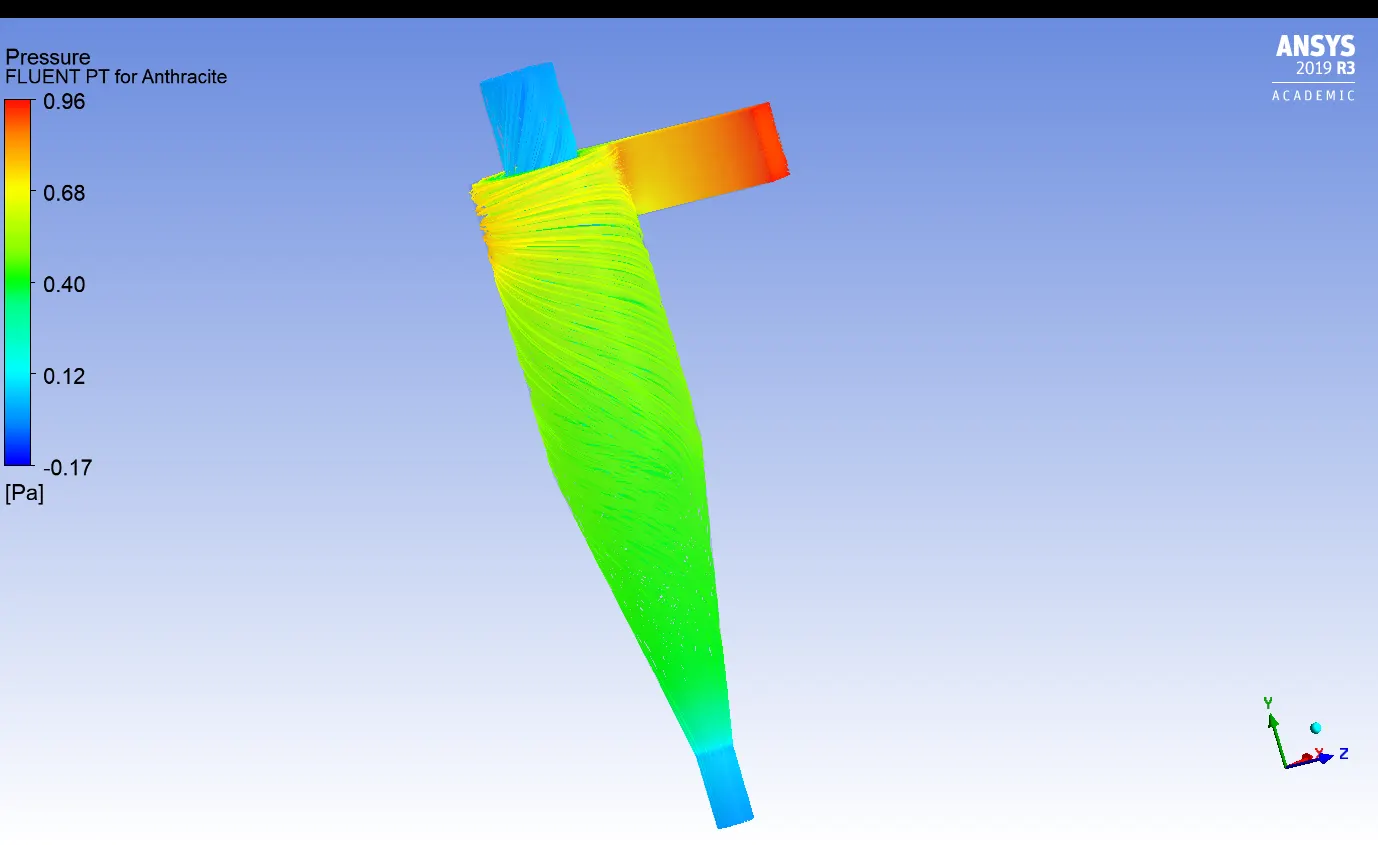
- Pressure
- Particle animation
Particle Info. :
| Tracked | Escaped | Trapped | Incomplete |
| 360 | 199 | 156 | 5 |
<<<<<<<<<<<<<<< [ For Velocity : 2m/s ] >>>>>>>>>>>>>>>
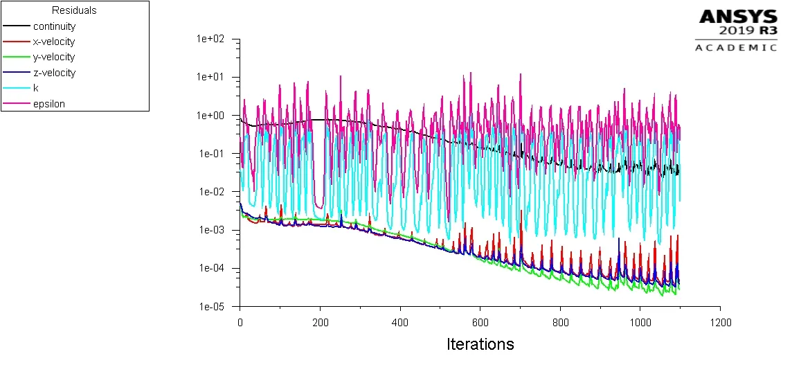
- Residual
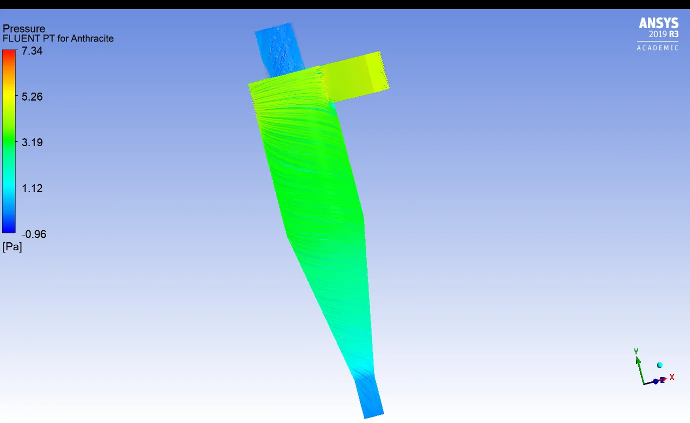
- Pressure
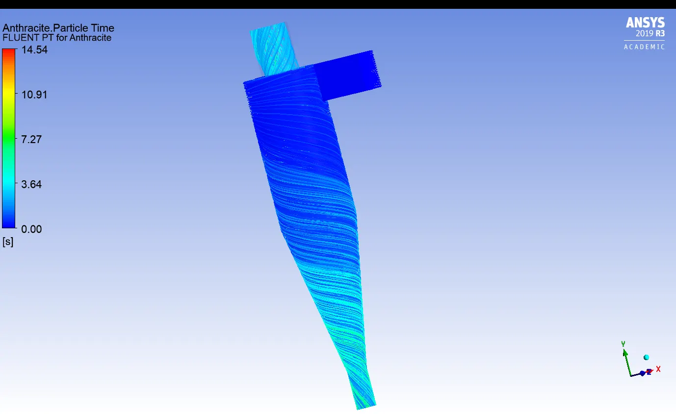
- Particle time
- Particle Animation
Particle Info. :
| Tracked | Escaped | Trapped | Incomplete |
| 350 | 116 | 230 | 4 |
<<<<<<<<<<<<<<< [ For Velocity : 3m/s ] >>>>>>>>>>>>>>>
- Residual
- Pressure
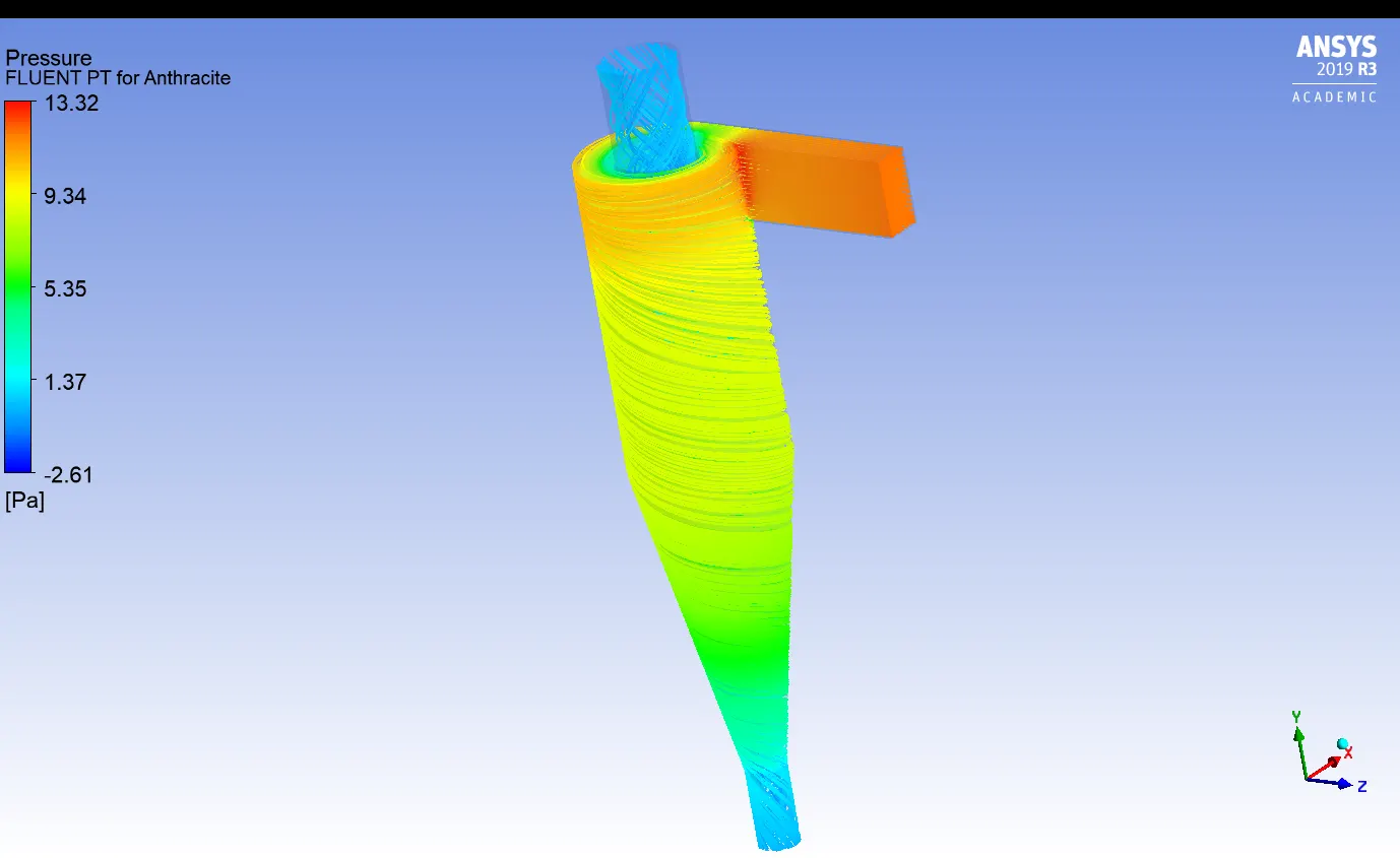
- Particle time
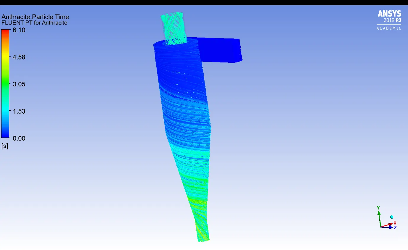
- Particle animation
Particle Info. :
| Tracked | Escaped | Trapped | Incomplete |
| 350 | 68 | 278 | 2 |
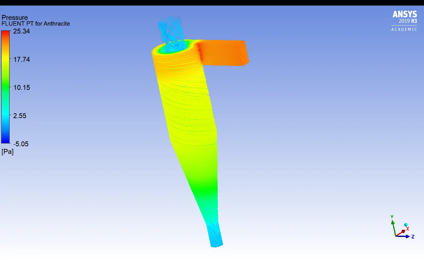
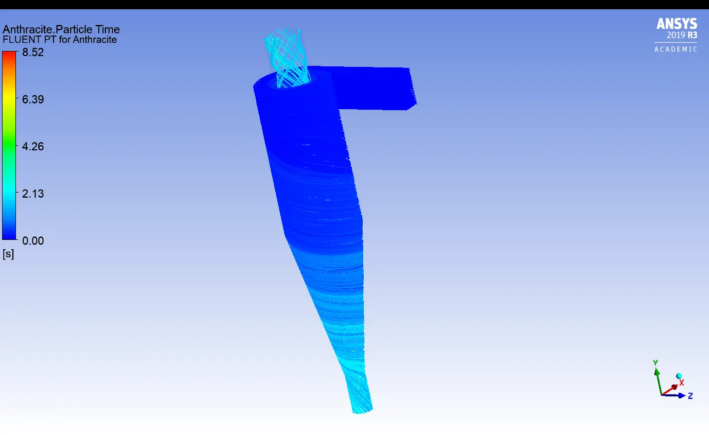
<<<<<<<<<<<<<<< [ For Velocity : 4m/s ] >>>>>>>>>>>>>>>
- Residual
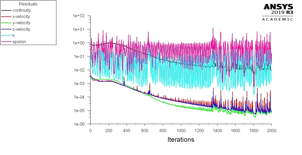
- Pressure
- Particle time
- Particle Animation
Particle Info. :
| Tracked | Escaped | Trapped | Incomplete |
| 350 | 38 | 311 | 1 |
<<<<<<<<<<<<<<< [ For Velocity : 5m/s ] >>>>>>>>>>>>>>>
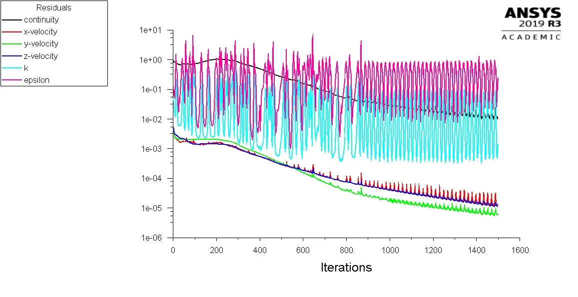
- Residual
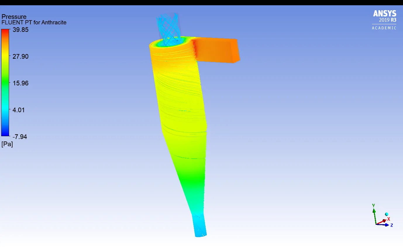
- Pressure
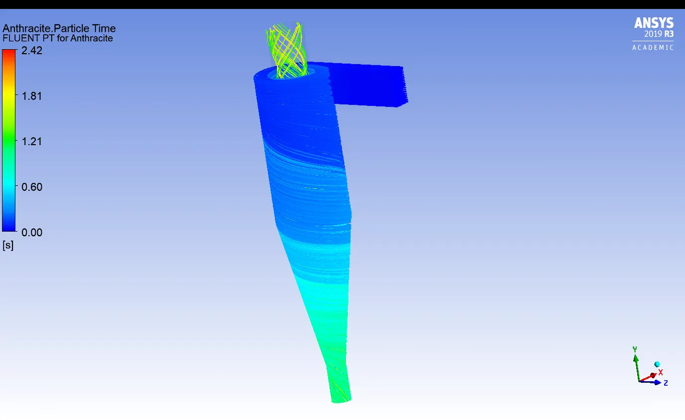
- Particle time
- Particle Animation
Particle Info. :
| Tracked | Escaped | Trapped | Incomplete |
| 350 | 31 | 319 | 0 |
Seperation Efficiency = (Particles Trapped/Particles Tracked) * 100
| Particle velocity | Trapped | Tracked | Efficiency | Pressure drop (Pa) |
| 1m/s | 156 | 360 | 43.33 | 0.9184 |
| 2m/s | 230 | 350 | 65.71% | 4.7434 |
| 3m/s | 278 | 350 | 79.42% | 11.9853 |
| 4m/s | 311 | 350 | 88.85% | 22.625 |
| 5m/s | 319 | 350 | 91.14% | 35.381 |
########################## { Observations } ##########################
- Finer mesh gives more no. of tracked particles, so finer the mesh more will be the accuracy of simulation as it tracks more particles.
- It can be seen that in CASE I as the particle diameter increases, no. of trapped particles increases too and so does the seperation efficiency.
- Also there is no difference in pressure drop in all sub cases of CASE I as the velocity is same for all sub cases.
- It can also be seen that, in CASE II as the velocity increases, so does the seperation efficiency and pressure drop.
- More no. of tracking steps results in more accurate and stable results, ultimately resulting in less no. of incomplete particle in critical cases.
- Also the floww seems to be converged as the residual repeats the same pattern after considerable amount of iterations.
Empirical models :-
1] Iozia & Leith model
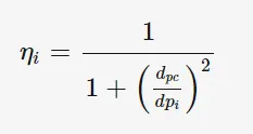
This model assumes that the particle carried by vortex, experiences 2 forces mainly centrifugal force and flow resistance. The collection efficiency for the same can be calculated by
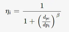
where dpi = particle diameter
dpc is the 50% cut size of Barth version.
2] Li and Wang model :-
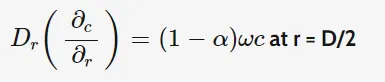
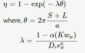
This model has partcile bounce and turbulent diffusion at cyclone walls. This model is based on following assumptions.
- The radial particle velocity and the radial concentration profile are not constant for uncollected particles within the cyclone.
- Boundary conditions with the consideration of turbulent diffusion coefficient and particle bounce re-entrainment on the cyclone wall are c=c0 at theta=0
-
The tangential velocity is related to the radius of cy-clone by:`uR^n=constant`
The collection efficiency for particle of any size can be calculated as follows :
- The tangential velocity of a particle is equal to the tangential velocity of the gas flow, i.e. there is no slip in the tangential direction between the particle and the gas.
- The tangential velocity is related to the radius of cyclone by: u R^n= constant.
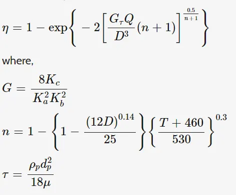
The efficiency can be calculated as follows :
4] Lappel model :-
- Lapple model was developed based on force balance without considering the flow resistance. Lapple assumed that a particle entering the cyclone is evenly distributed across the inlet opening.
- The particle that travels from inlet half width to the wall in the cyclone is collected with 50% efficiency.