CHT Analysis on Exhaust port
AIM-:
Study of CHT (EXHAUST PORT) maintaining proper Y+ value
THEORY
Conjugate Heat Transer :
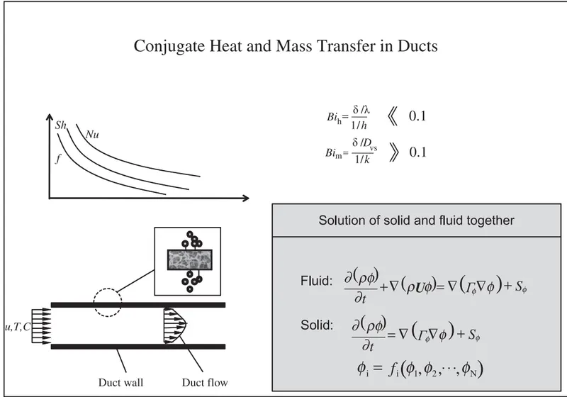
Conjugate heat transfer corresponds with the combination of heat transfer in solids and heat transfer in fluids. In solids, conduction often dominates whereas in fluids, convection usually dominates.
In simple words, it is the heat transfer between solid and fuild simultaneously. There is a thermal coupling at the interfaces of two regions.
Conjugate heat transfer is observed in many situations. For example, heat sinks are optimized to combine heat transfer by conduction in the heat sink with the convection in the surrounding fluid.
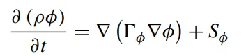
The general form for fluid flow, heat, and mass transport in the fluid (air or liquid) duct can be expressed by

where t is time (s), ρ is fluid density (`(kg)/m^3`), φ is a general variable which can be velocity, temperature, or concentration, U is the velocity vector matrix, `Gamma_phi` is generalized diffusivity, and `S_phi` is a generalized source term. Function `"div"` is divergence, and grad is the gradient vector. It can also be expressed as

If`Gamma_phi` is a constant, then

where`nabla^2` is the Laplace operator.
For ducts in heat and mass exchangers, the solid walls are usually too dense to form a macroscopic fluid flow inside. So the macroscopic fluid flow in the solid is ignored. Heat and mass diffusion in the solid can be expressed by a general form as
Why CHT :
Understanding of the complex heat transfer mechanisms and the interactions between those mechanisms to improve the performance and increase the lifespan of the components to be analysed.
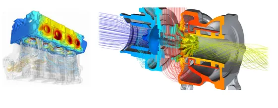
Conjugate Heat Transfer analysis provides the temperature distribution in solid and fluids, and clear insight on velocity distribution and mechanism of heat transfer of fluid, like in engines.
It is more accurate and fast to simulate the problem.
Can be used in complex scenarios like in automotive components or in power plant components.
Multiple number of regions can be simulated.
All types of region combination can be simulated like solid-fluid,fluid-fluid, etc.
Where is CHT analysis done :
Analysis of Heat transfer mechanism in turbocharger.
HVAC systems
Burners, combusters, electronic devices.
Automotive, power plants and various other applications.
Heat transfer in ribbed passages
Heat transfer in micro-channels
Heat transfer in fin arrays
Heat transfer in mobile phones
Drying of a porous flat plate
Simulation Model :
Simulation precedure :
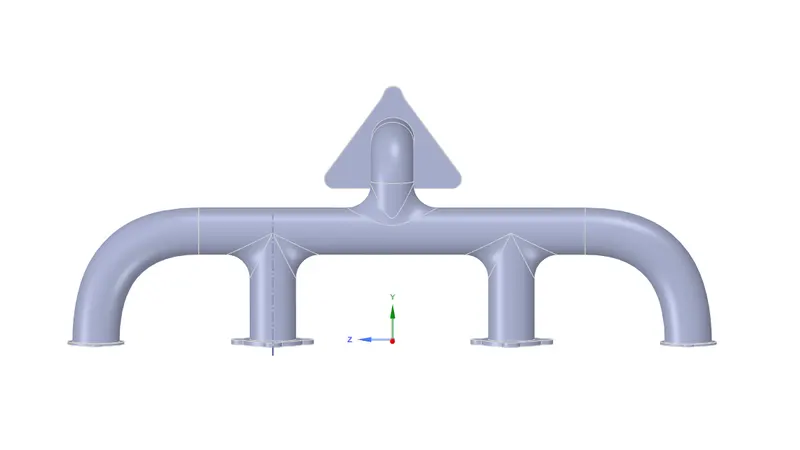
We are going to simulate the exhaust port with baseline and refined mesh.
Geometry :
1. Import the model of exhaust port.
2. Go in repair and clear the extra edges if any.
3. Then go in prepare and extract the inner volume.
4. After that select solid and fluid component move them to new componet.
5. Finally go in workbench and select shareprep and also share the topology in desing.
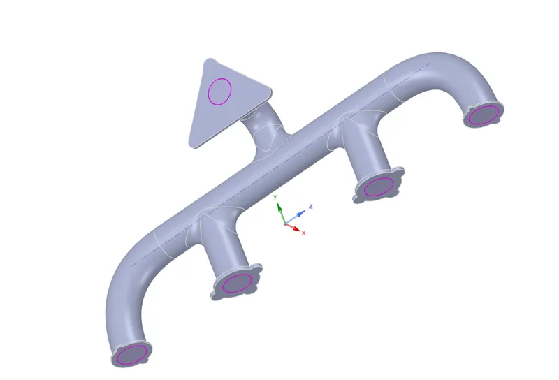
N.B-: Pink colour border tells that solid-fluid volume shared correctly
Mesh :
1. Open the mesh section in workbench.
2. First name the faces which are inlets, outlet, outer-wall-convection.

3. Then mesh the geometry
Element size- .15mm
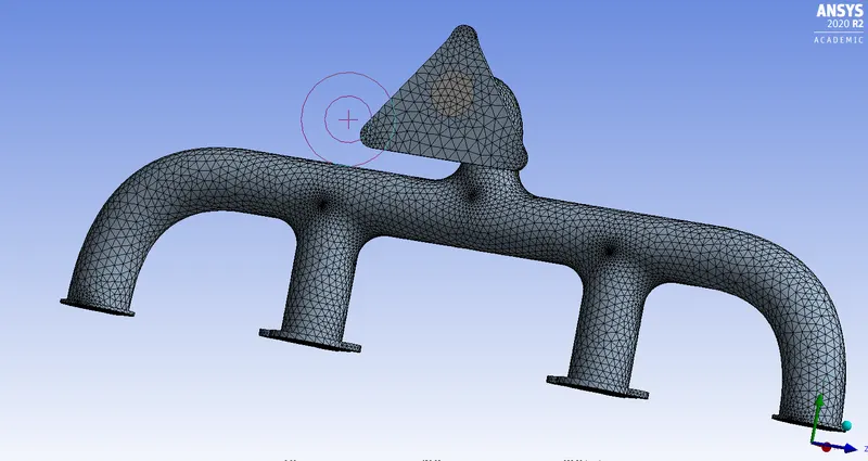
4. Check Mesh quality

Setup :
1. Perform the mesh check.
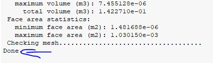
2. Turn on the energy equation and viscous model.
3. Set up the materials, solid and fluid one.
4. Then set up the boundary conditions like inlet velocity, outlet pressure, outer wall convection's HTC.
Inlet
velocity-5 m/s
Tempereture- 700°C
Outlet
Gauge presure- 0 pa
Outer wall convection
wall heat transfer co-efficient (h)= 20k
velocity- No sleep
wall-solid-fluid-solid_volume
No sleep
Heat flux - 0°C
Adiabatic
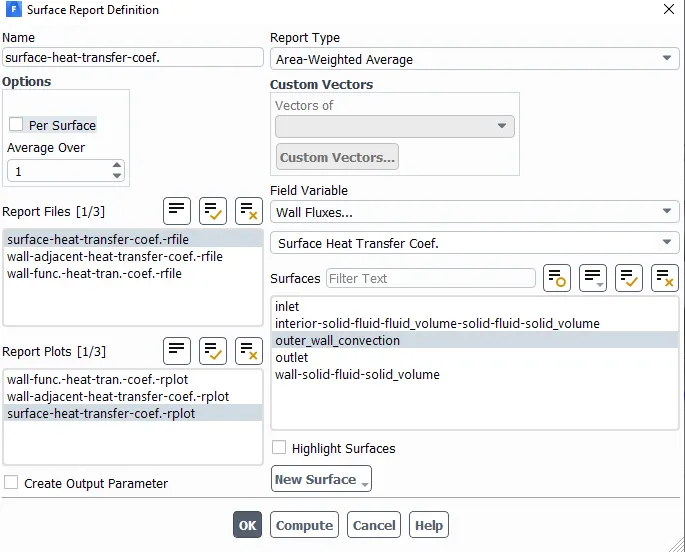
5. Also set up the solution method and report definitions.
solution method-
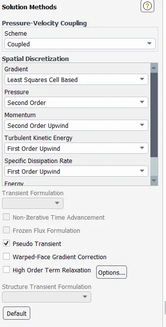
Defination
6. Then initialize the problem with hybrid initialization.
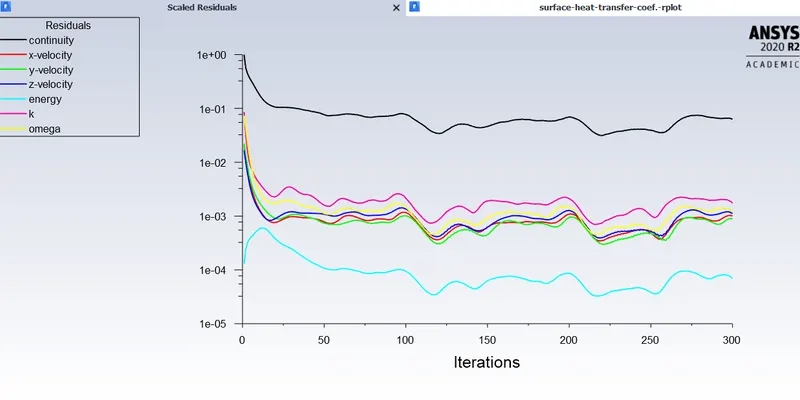
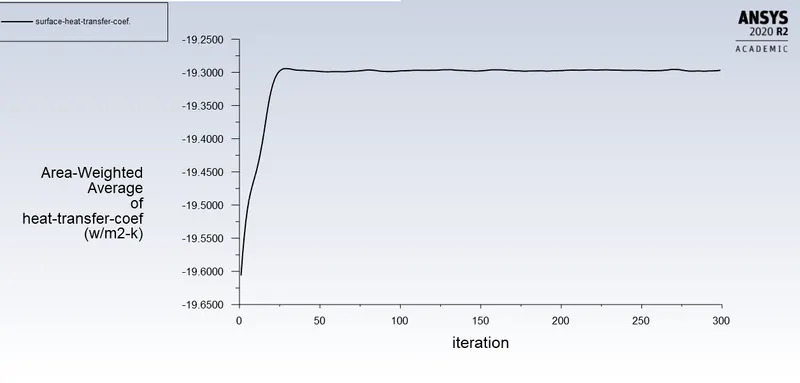
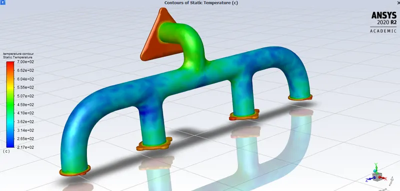
7. After that set the Contours and solution animation and run the case with some iterations and observe the same.
Result :
1. Select the outer wall volume to make it visible. Also color it with the variable needed to be observed
2. Insert the plane and color it with variable like Temperature and Velocity which shows the Temperature and Velocity flow on plane.
3. Edit the legend according to requirement. This completes the results and hence the entire simulation.
TEMPERATURE
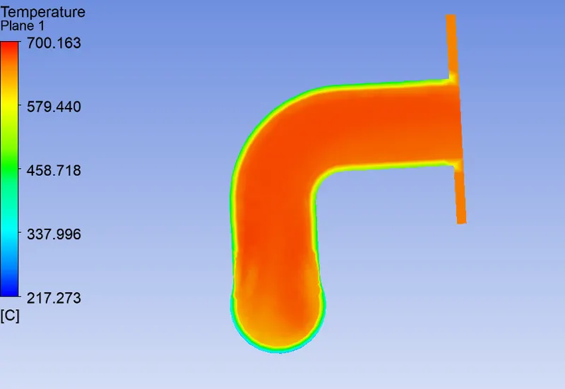
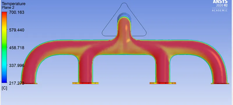
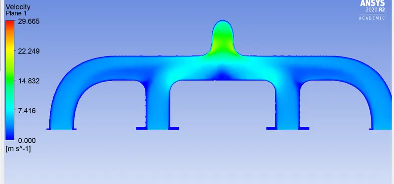
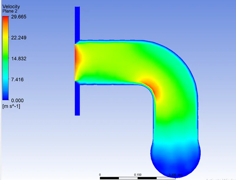
VELOCITY
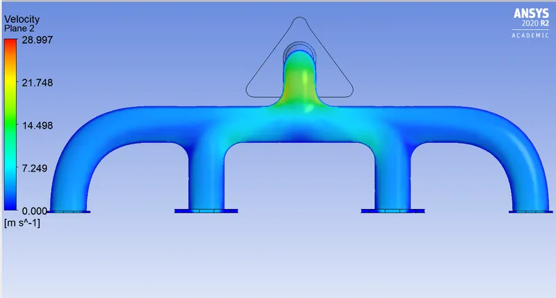
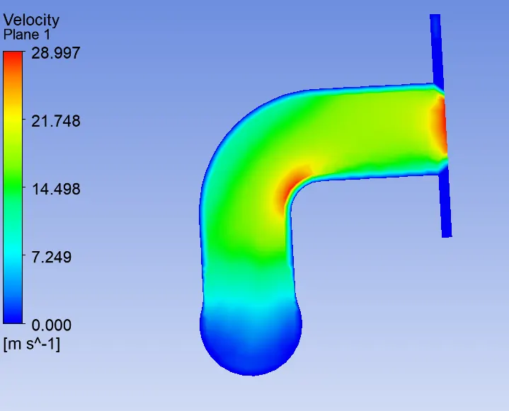
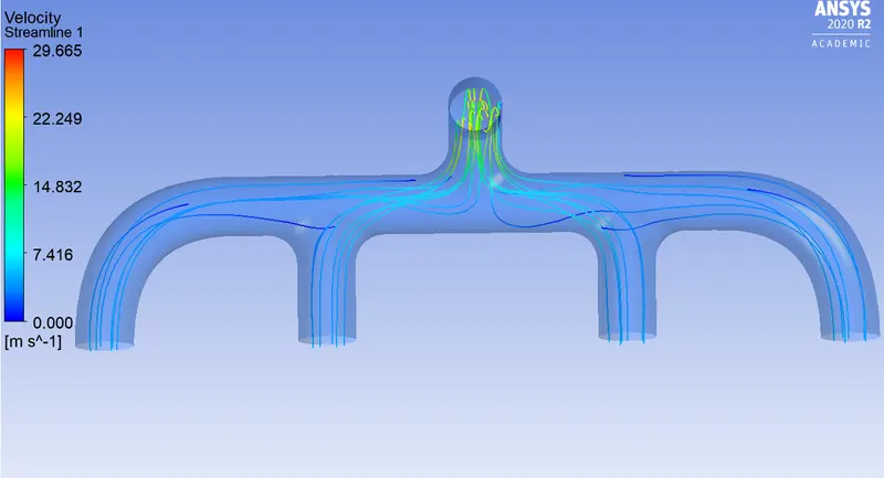
VELOCITY STREAMLINE
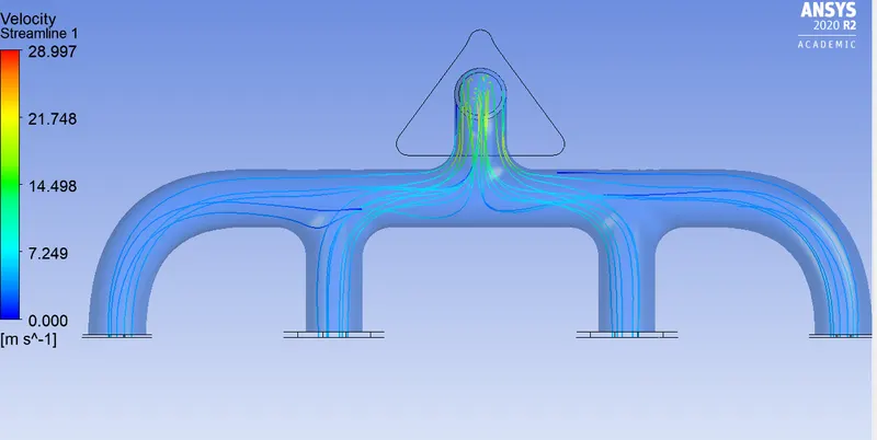
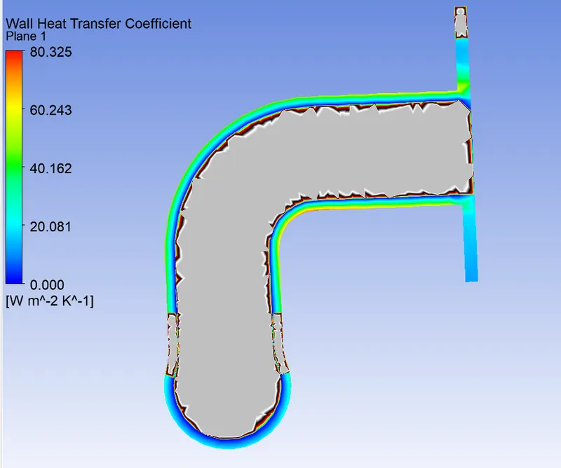
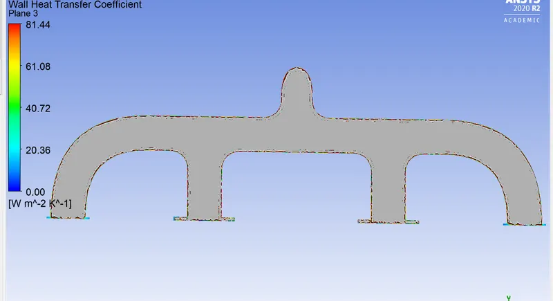
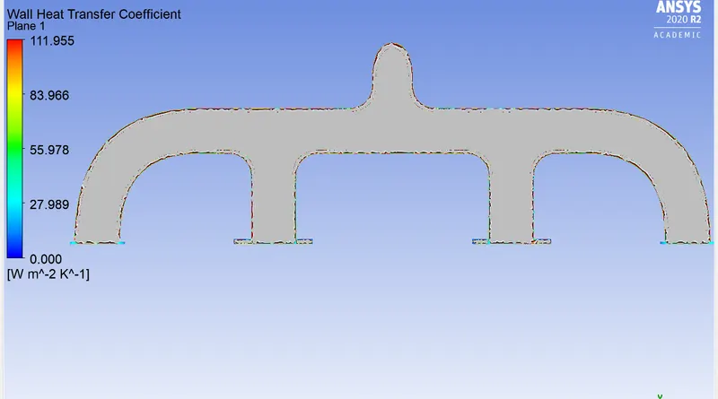
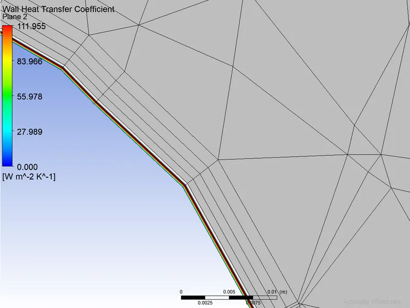
WALL HTC
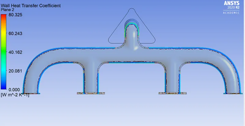
N.B-: Same procedure followed for the cases mentioned below.
CASE - 2
MESH- .15 mm
Turbulence model- K-Omega (SST)
solution method- Simple (Default parameter)
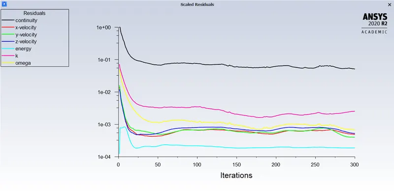
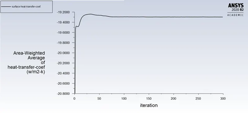
Residual plot
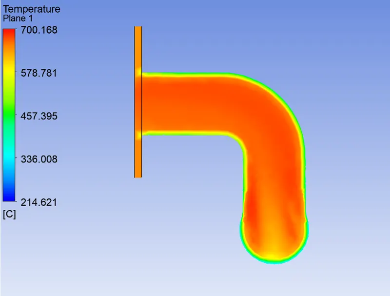
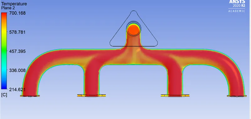
TEMPERATURE
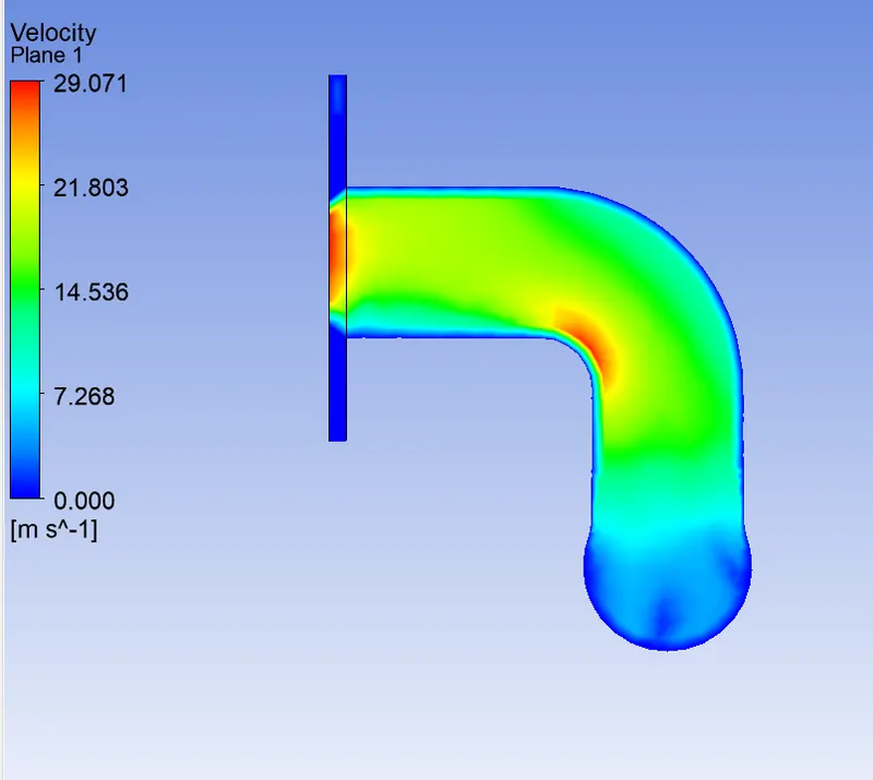
VELOCITY
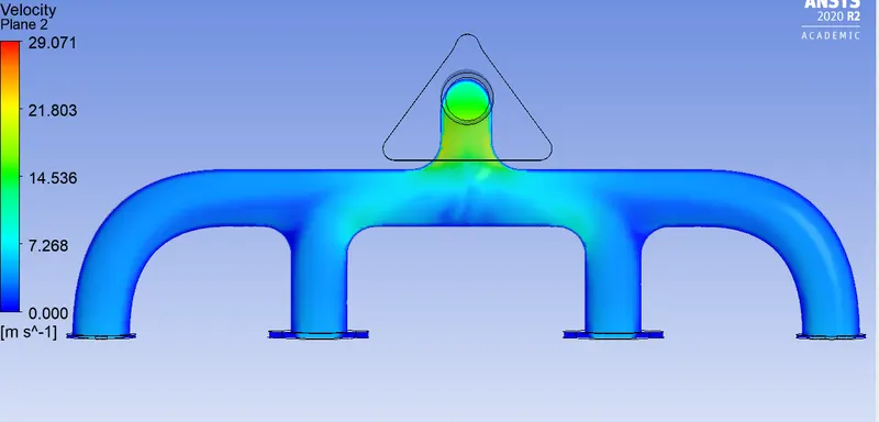
VELOCITY STREAMLINE
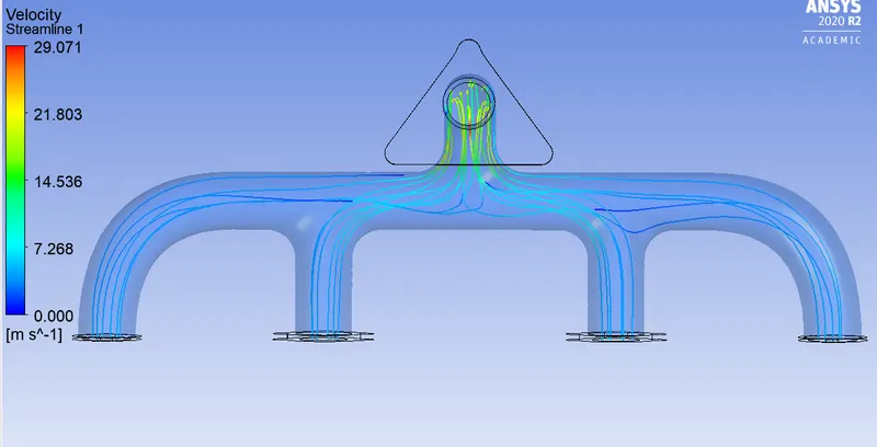
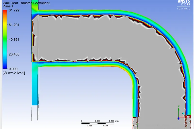
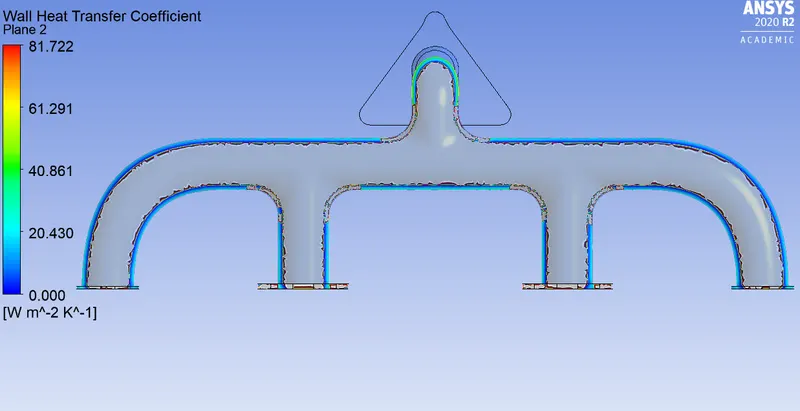
WALL HTC
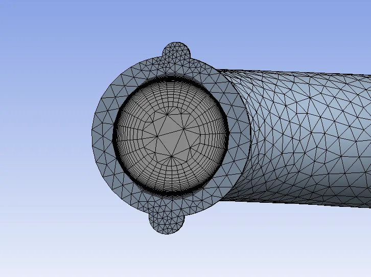
CASE-3
MESH- 25mm
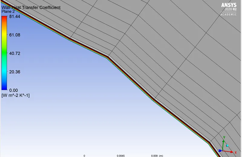
First layer height - .56mm
maximum layer -15
growth rate - 1.2
Turbulence model- K-Omega (SST)
solution method- Simple (Default parameter)
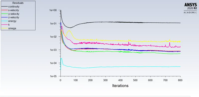
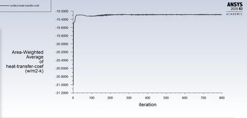
Residual
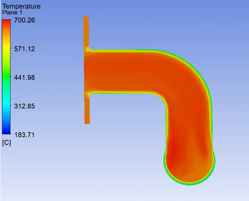
TEMPERATURE
VELOCITY
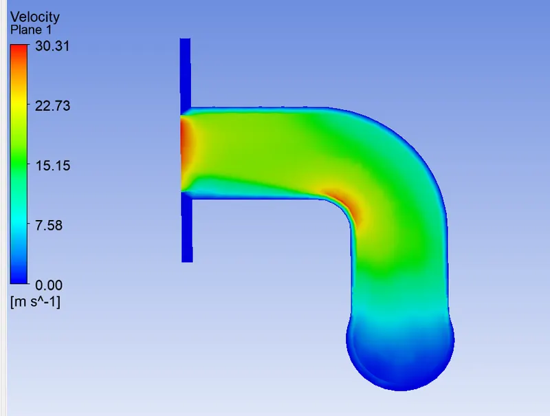
VELOCITY STREAMLINE
WALL HTC
Case-4
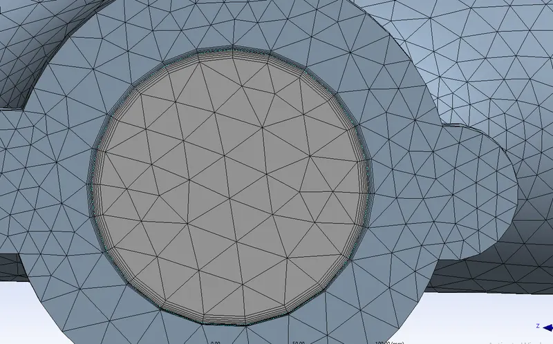
MESH- .15 mm
Total thickness - 5mm
maximum layer - 5
growth rate - 1.2
Turbulence model- K-epsilon (standard)
solution method- coupled (Default parameter)
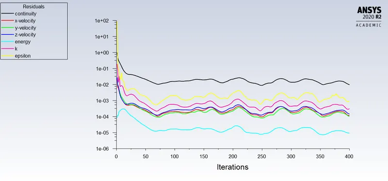
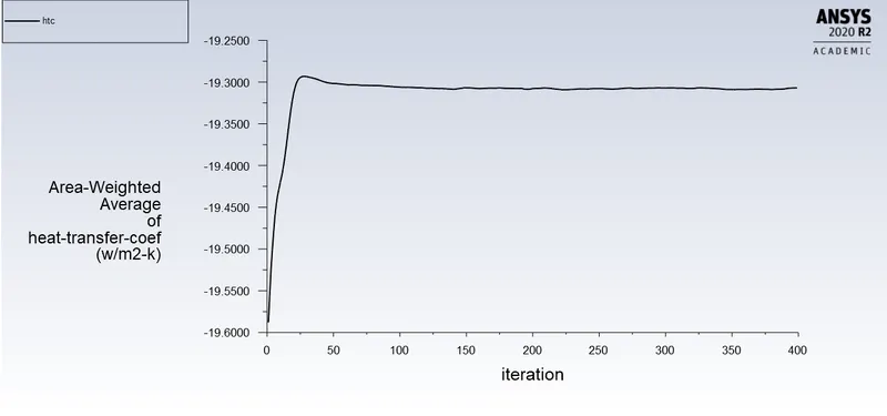
Residual plot
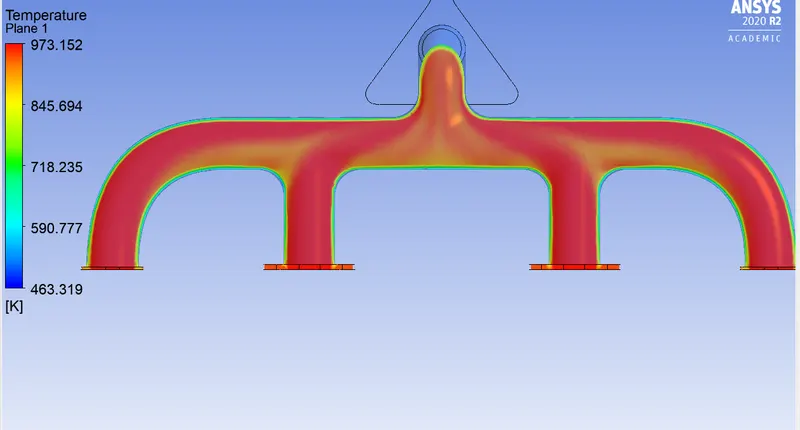
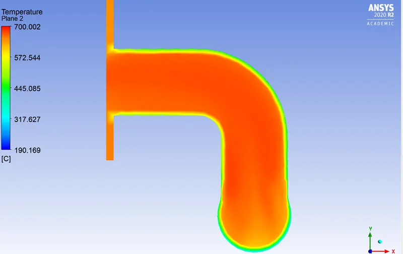
TEMPERATURE
VELOCITY
VELOCITY STREAMLINE
WALL HTC
Verify HTC :
Under forced convection circumstances, we can determine the heat transfer coefficient by using the Dittus-Boelter
correlation. Using the Dittus-Boelter correlation the heat transfer coefficient can be calculated in the following way using
two further dimensionless groups, the Reynolds number and the Prandtl number:
h = (k/D )*Nu
where k is the thermal conductivity of the liquid, D is the Hydraulic diameter, and Nu is the Nusselt Number which is
determined by the following equation:
Nu = 0.023Re Pr
where, n= 0.4 when fluid is being heated
n= 0.3 when fluid is being cooled
In this equation, Re is the Reynolds number which equates to:
Re = (m D )/(μ)
and Pr is the Prandtl number :
Pr = (CP* μ)/k
For the Reynolds number, m is equal to the mass flow rate. For the Prandtl number, CPis equal to heat capacity, and in both
equations, μ is the viscosity of the fluid in consideration. Once we have all of these factors, we can get a decent
estimation of the heat transfer.
Also we can get the estimation from some published papers or from some experimental values.
Accuracy of HTC prediction :
Accuracy of the predictions depends on several things like,
1. Accurate geometry of model.
2. Its Mesh quality.
3. Inflation layers
4. Properties of material being used.
5. Turbulence models.
Conclusion :
1. From the above both cases output, we can say that the results are almost same but the refined mesh gives us more smoothness and accuracy.
2. Two factors influence the performance simultaneously: (a) Flow is developing along the length and the heat transfer coefficients tend to decrease along flow (b) Turbulence;
3. At the same time, turbulence is developing with tube rows at bent, which would increase heat transfer coefficients.
4. The maximum heat transfer results at bend of exit port, It is because to ensure conservation of mass at exit port velocity should more, which resuts in higher velocity and increse in velocity attain a Reynolds number that is sufficient to make flow trurbulent and higher Nusselt number at pipe bent at exit, which increses Heat transfer co-efficient at that loicaton.