CHT Analysis on a Graphics card
AIM-: Numerical study of forced convection heat transfer from rectangular fins at different Reynolds numbers
Theory-:
Efficient cooling of high power electronics allows miniaturization and faster and more powerful electronic systems. Most heat exchangers, microelectronics devices, and embedded systems are cooled using forced air convection employing heat sinks and fans . The sizing of the cooling system is crucial for miniaturized devices as it impacts the size, weight, and acoustics. In these systems, the flow can be laminar, transitional or turbulent at low Reynolds number, `Re = ( U_infty*D)/nu`, where U∞ is the flow velocity, `D_h` is the hydraulic diameter, and`nu` is the kinematic viscosity of the fluid. This definition of Re is used throughout the project. In design situations, the choice between natural and forced convection can significantly affect the cooling performance, cost, size, and reliability of the device. The most commonly used heat sinks for cooling circuit boards in power electronics devices, have rectangular straight fins, through which air is forced parallel to the fins (In our case it is normal to fins). Rectangular straight fins are the simplest to manufacture, by extrusion at low cost. Heat transfer occurs across the thermal boundary layer as a result of differential heating of fluid around the fin surfaces. In order to design efficient forced cooling systems, it is necessary to establish a relationship between the flow and the fin geometrical parameters so that heat transfer can be maximized for minimum fan power and size of heat sink.
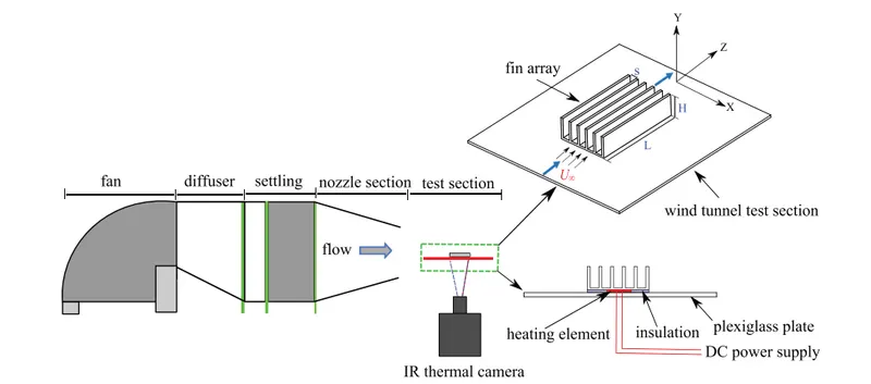
N.B- The purpose of this project is to characterize the forced convection heat transfer from a rectangular straight fin array with the incoming flow normal to the fin channels at various Reynolds number. The novel feature of this investigation is its focus on short fin channels, with hydrodynamically and thermally developing flow.
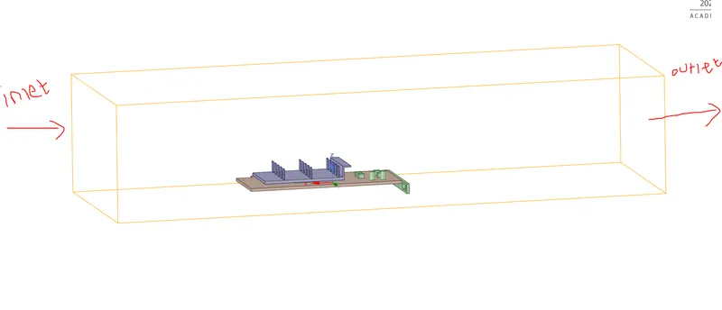
Computational model
We analyze the heat transfer and flow field using steady state conjugate three-dimensional flow simulations. The computational fluid dynamics solver ANSYS-Fluent was used for the simulations.The governing equations are the conservation of mass, momentum, and energy for the flow, and the heat conduction equation for the solid, which are written in Cartesian co-ordinates, with x transverse to the fins, y in vertical direction, and z in the direction of the fins and the flow, as follows.
Continuity equation for the steady, incompressible flow:
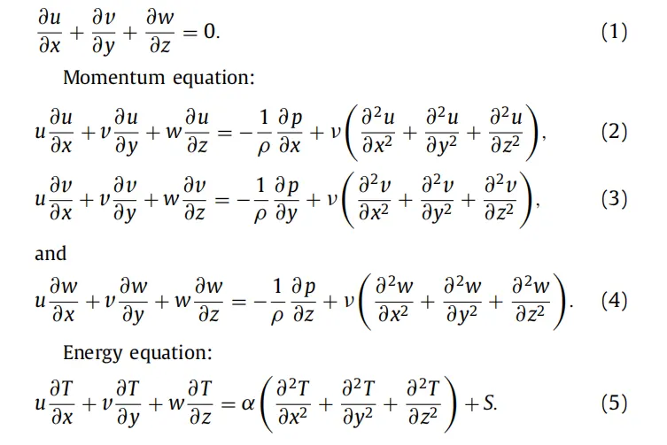
where S is the source term for radiation( ignored in our case). The heat conduction equation ( ignored in our case) for the fins was the Laplacian. It is noted that “conjugate” heat transfer means continuity of heat flux between solid and fluid.
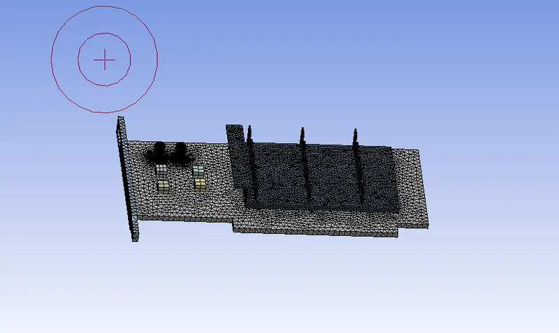
The computational domain was discretized with fully structured tetra grids with high resolution in the near wall region to capture the effects of thermal boundary layer more accurately. A typical computational mesh used in the simulation is shown in mesh section of each case.
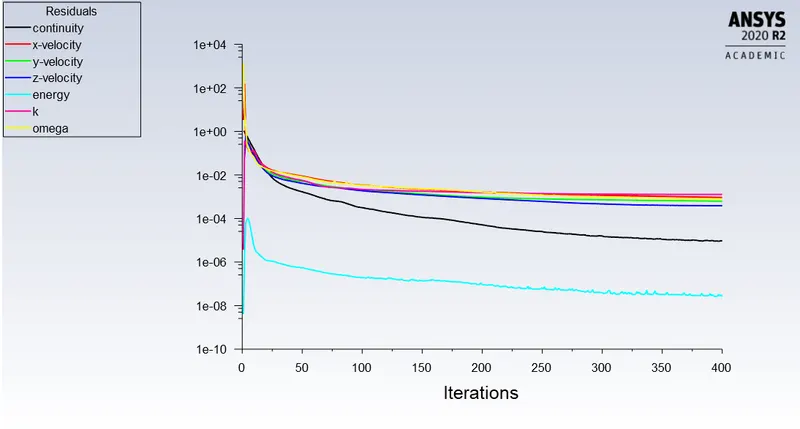
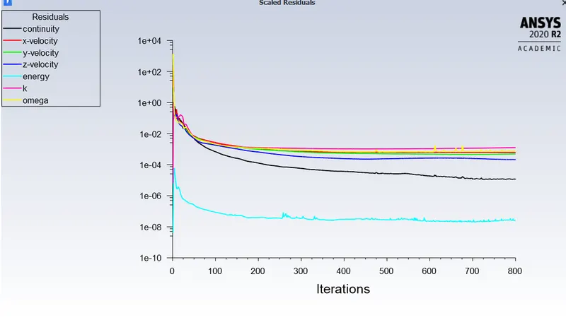
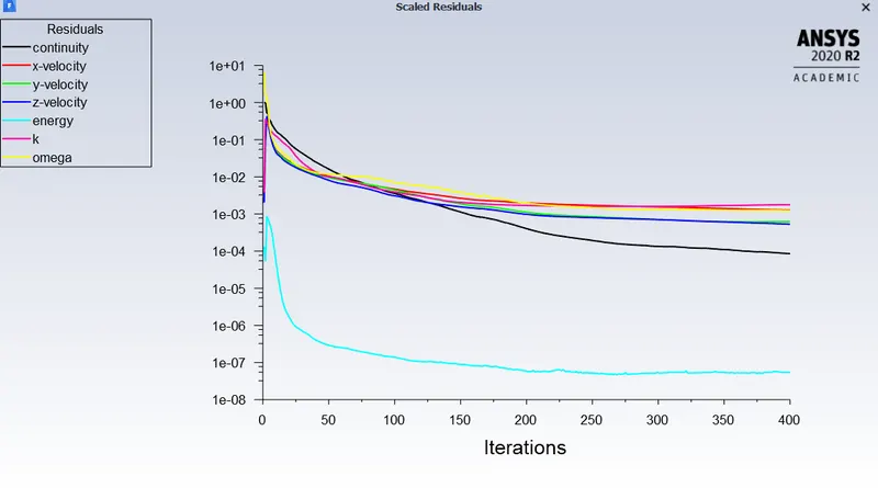
A control-volumebased technique was used to discretize the governing equations. A second-order up-winding scheme was used for more accuracy. Convergence criteria of 10−4 for the flow, and 10−7 for the energy were used. At the inlet, the free-stream velocity (1m/s, 3m/s, 5m/s) and outlet is prescribed as shown in figure-1.
The properties of inlet air used in the simulations were: density ρ = 1.2096 kg/m3, specific heat capacity `C_p` = 1005 J/kgK, viscosity μ = 1.915×10⁻⁵ kg/ms, thermal conductivity k = 0.0261 W/mK, and molecular weight 28.966 kg/k mol.
No-slip walls were specified for the fin surface boundary condition. To confirm that the computational domain was adequately resolved and numerical uncertainty was small, a grid independence study was conducted by gradually refining the grid size until an acceptable convergence was achieved for the maximum fin temperature, which is summarized in setup section figure.
we used the Reynolds-averaged form of these equations, which contain the Reynolds stresses and heat fluxes. For brevity, we omit the equations as they can be found in standard references, (Mentioed below). For the transition-turbulent regime, we used the SST k − ω model and K-epsilon. All cases were computed with the standard model constants. The results are summarized in solution section.
The heated fin array on a horizontal surface with a free-stream directed normal to the channels represents a situation where buoyancy forces may influence the development of a forced convection boundary layer. The buoyancy force acts vertically upward, which is perpendicular to the direction of the free stream.
Case set-up in ANSYS-FLUENT
Geometry :
1. Open the geometry section and import the given Graphics card geometry.
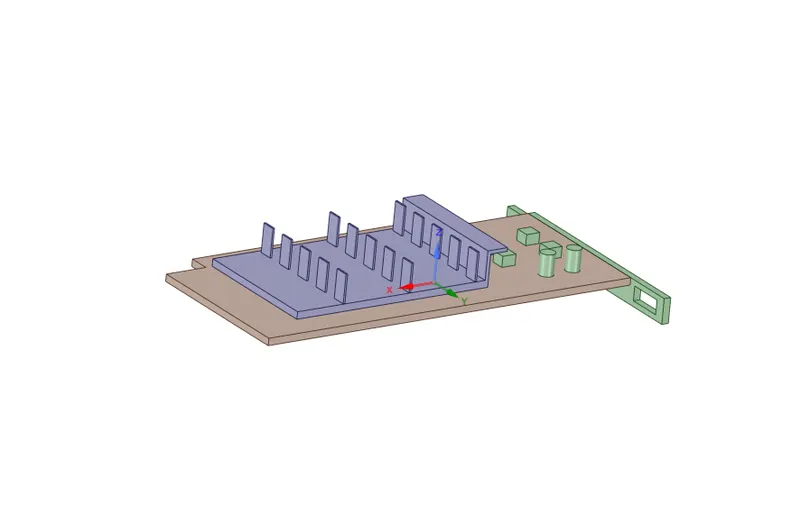
2. Turn on share topology

Mesh :
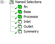
1. Open the mesh and name the boundaries like Inlet, Outlet, Symmetry.
2. Now, generate the default mesh provided.
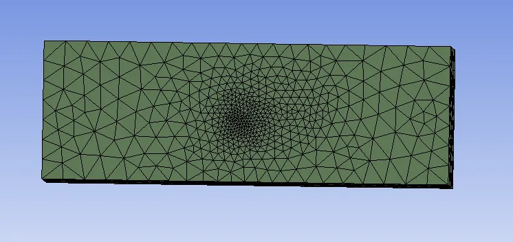
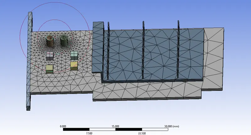
3. By default, Fluent analyzes the hot spots and meshes them accordingly.
4. Here we have used body sizing for the processor as the default element size was not able to capture the heat generation(it
showed just 4 elements on processor)
Setup :
1. Open the Setup and perform the mesh check.
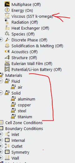
2. Then set the pressure based solver and turn on the the energy equation.
3. Set the viscous model( we have used k-omega SST model).
4. Now set the materials for fluid and solid according to requirement.
5. Now from cell zones assing the solid and fluid zones(We have selected fuild for the enclosure and solid for Base,
processor, fin).
6. In same cell zone section set the energy (5e7 Wt/m^3) source for the processor so that the processor emits the energy.
7. Set the Boundaries like inlet velocity.(Here we have simulated the problem for 3 Velocities i.e. 1,3,5 m/s for both Baseline
and Refined mesh).
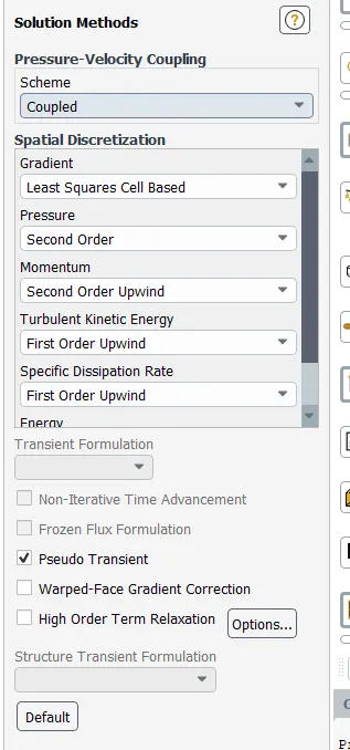
8. Now set up the solution method(we have used Coupled Scheme with first order approx).
9. After that initialize it with hybrid initialization and set a plane to view the contours on it.
10. Finally set the velocity and temperature contours and run the simulation.
CFD POST
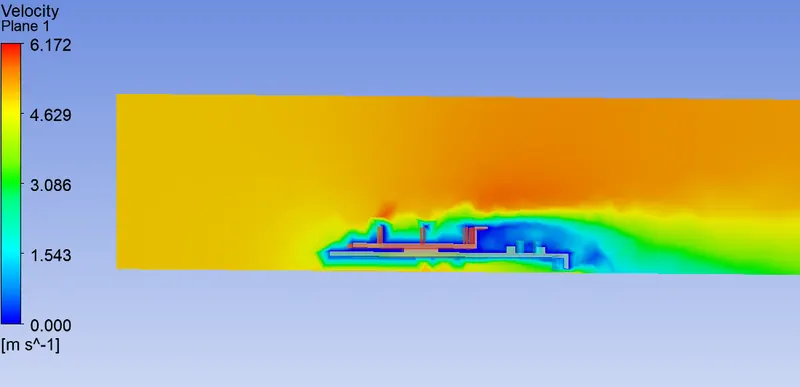
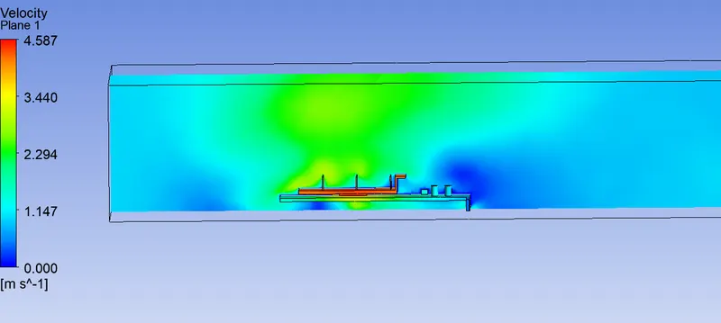
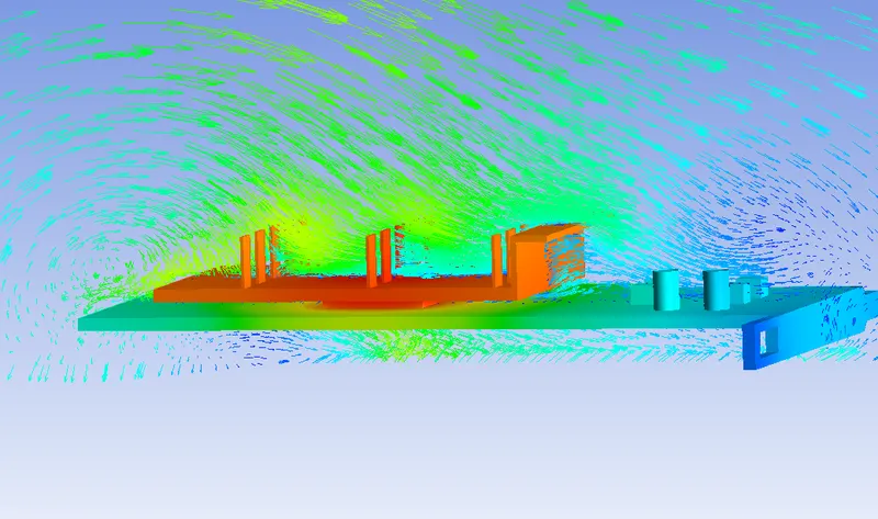
1. Open the Results section and create a plane to observe the velocity over entire graphics card.
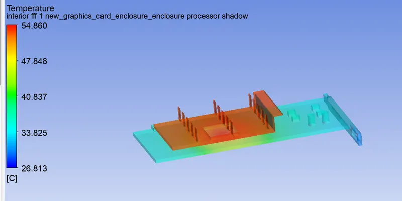
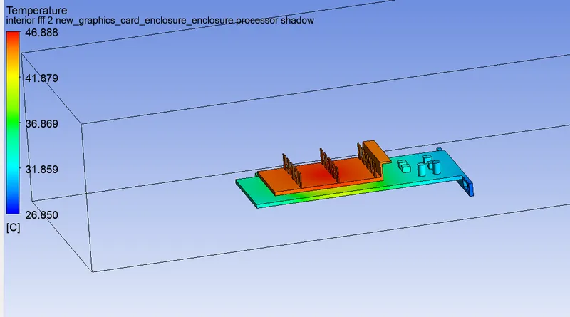
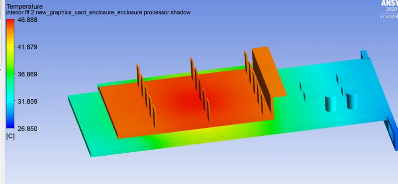
3. We will observer the temperature distribution over solid base, processor and fin.
Case-1
v = 1m/s
MESH- Refined
Turbulence Model - K-w
convergence plots.
Results
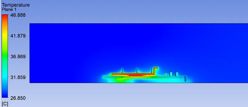
TEMPERETURE
Velocity
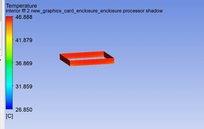
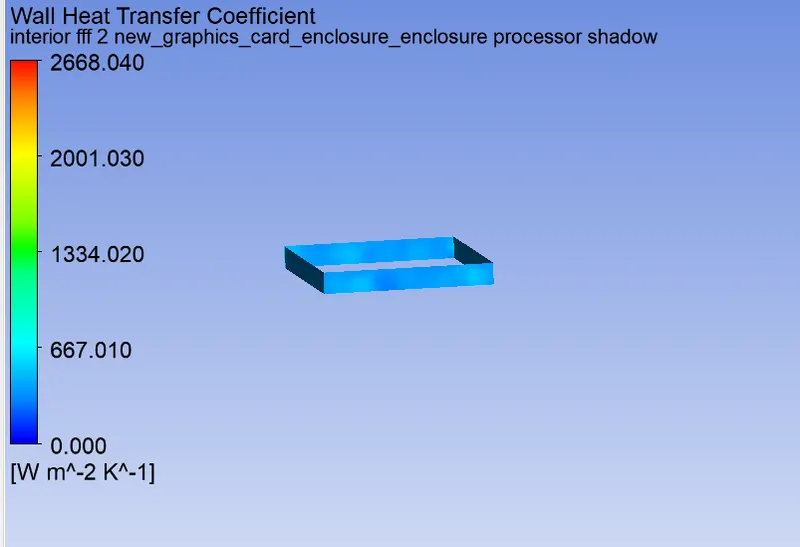
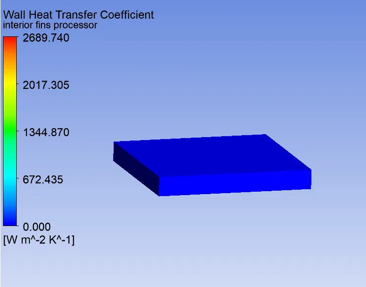
Maximum temperature and heat transfer coefficient attained by the processor.
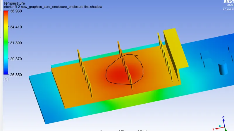
Hotspots on the model
Case-2
v = 3m/s
MESH- Refined
Turbulence Model - K-w
convergence plots.
Results
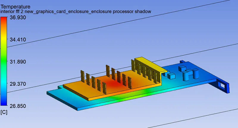
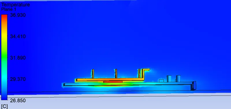
TEMPERETURE
Velocity
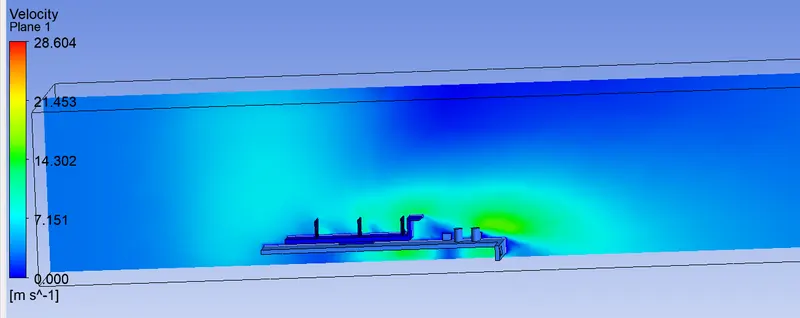
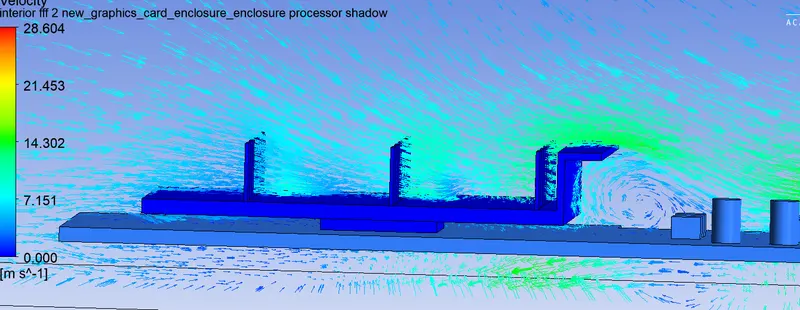
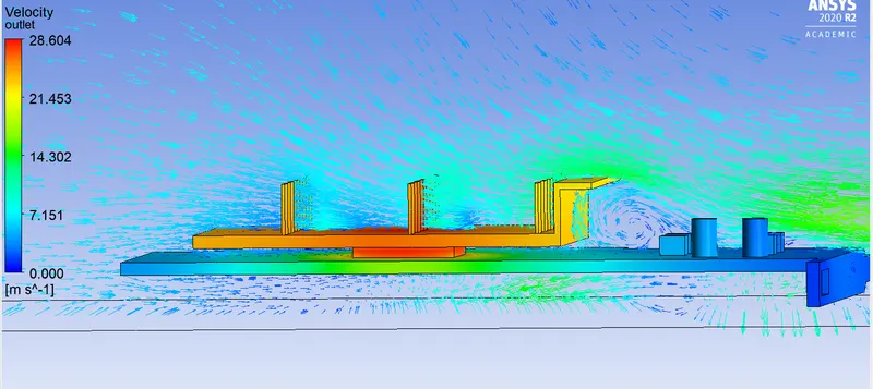
(vel+temp)
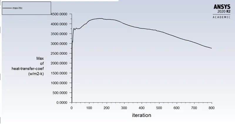
Maximum temperature and heat transfer coefficient attained by the processor.
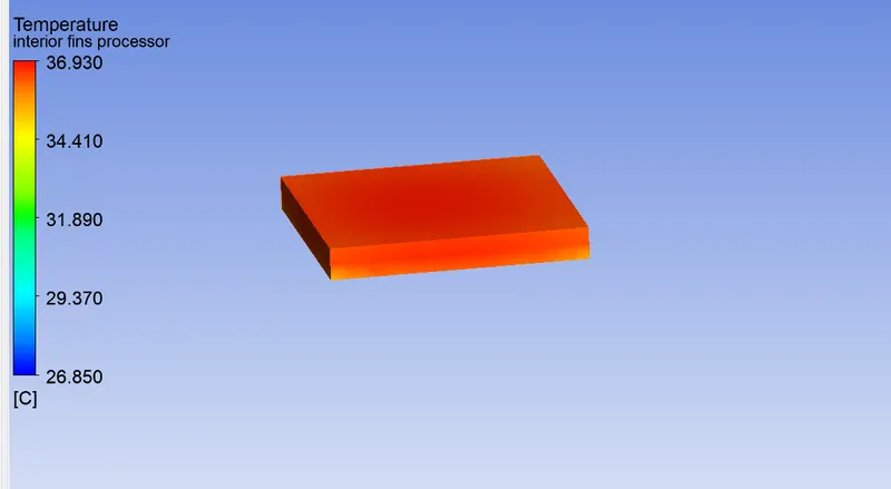
Hotspots on the model
Case-3
v = 5m/s
MESH- Refined
Turbulence Model - K-w
convergence plots.
Results
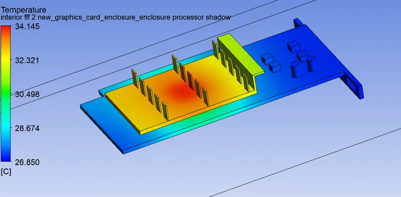
TEMPERETURE
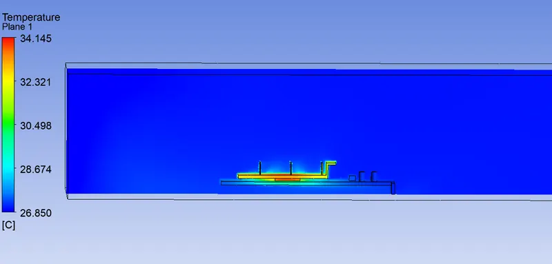
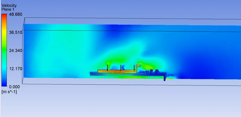
Velocity (vel+temp (base fin processor)
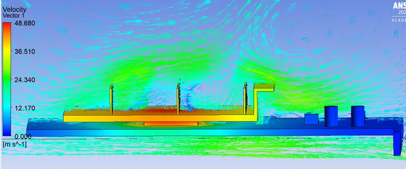
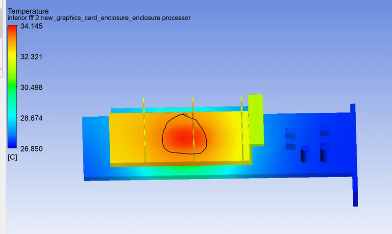
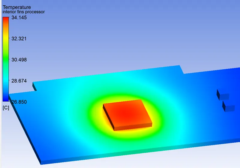
Maximum temperature and heat transfer coefficient attained by the processor.
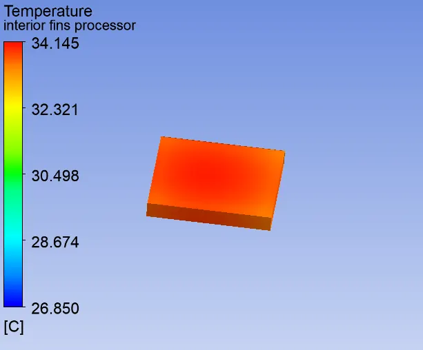
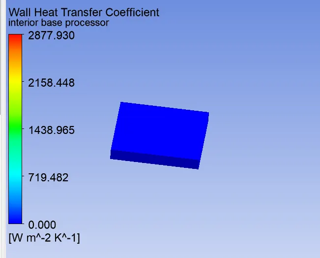
Hotspots on the model
Conclusion
1. Tempereture plot shows that the temperature of the air above the fin top for the case -3 of maximum heat transfer and U∞ = 5 m/s, is close to ambient, indicating that natural convection is negligible.
2. Near the leading edge of the channels, the buoyancy is negligible as the viscous forces dominate for case-1 and 2, and then further downstream the viscous forces diminish and the buoyancy may increase due to the heated air. Thus the effect of natural convection is assumed negligible for the case investigated here as U∞ ≥ 5 m/s .
3. Without radiation, the maximum temperature increased to 34.145 ◦C (for case-3), indicating that the contribution of radiation is small for the specific fin design and the range of inlet flow conditions and maximum fin temperature investigated here.As the heat transfer depends on the flow field, turbulence intermittency, air velocity, and temperature distributions in the fin channels are examined for different cases.
4. At low Re, it is observed that the flow is transitional toward the exit of the channels , and at higher Re, the flow is transitional at about halfway along the channel and becomes more turbulent toward the exit of the channels . Given the extent of transitional flow at the lowest and highest Re, it is surprising that the overall Nu results do not show strong sensitivity to flow state.
5. Air velocities at mid-section along the fin channel at different heights from the fin base for the case, U∞ = 5 m/s at are plotted in case -3 . It is seen that the velocity in the channels near the fin tip is approximately equal to the 5 times inlet air velocity U∞, indicating that the flow is highly influenced by the fins.
6. Because of recirculation region case-2 has aparently more heat at downstream of fin. That recirculation region can be seen in velocity vector plot in case 2.