Week 8 - Simulating Cyclone separator with Discrete Phase Modelling
SIMULATING CYCLONE SEPARATOR
Aim:- To perform analysis on cyclone separator and calculate the separation efficiency and pressure drop.
Objective:-
- To write a few words about any four empirical models used to calculate the cyclone separator efficiency.
- PART 1 :To perform an analysis on a given cyclone separator model by varying the particle diameter from 1 μm to 5 μm and calculate the separation efficiency in each case. Discuss the results. [Use both the velocity's as 3m/sec.]
- PART 2: To perform an analysis on a given cyclone separator model by varying the particle velocity from 1 m/sec to 5 m/sec and calculate the separation efficiency and pressure drop in each case. Discuss the results. [Use particle diameter size as 5 μm for all cases & keep flow velocity same as particle velocity]
Boundary Conditions:-
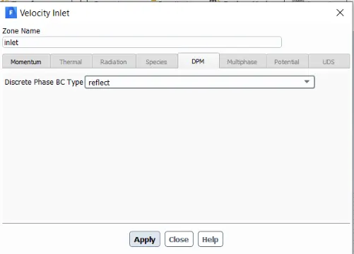
Inlet and wall:- Reflect
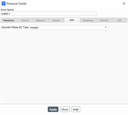
Outlet(Top):- Escape
Outlet(Bottom/dustbin) - Trap
Theory :
Cyclone Separator
Cyclone separators are separation devices that use the principle of inertia to remove particulate matter from flue gases.Those are the devices built to remove particular matter larger than 10micro meter .Therer are also few effective cyclone separators that can be remove as short as 2.5 micro meter .This is usually an inexpensive device . Cyclone separators is one of many air pollution control devices known as pre-cleaners since they generally remove larger pieces of particulate matter. This prevents finer filtration methods from having to deal with large, more abrasive particles later on.
The size of the cyclone depends largely on how much flue gas must be filtered, thus larger operations tend to need larger cyclones. For example, several different models of one cyclone type can exist, and the sizes can range from a relatively small 1.2-1.5 m tall (about 4-5 feet) to around 9 meters (30 feet)—which is about as tall as a three-story building.
Working of Cyclone Separator
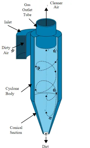
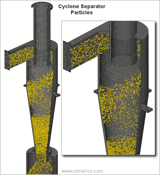
cyclone separators work much like a centrifuge, but with a continuous feed of dirty air. In a cyclone separator, dirty flue gas is fed into a chamber. The inside of the chamber creates a spiral vortex, similar to a tornado. The lighter components of this gas have less inertia, so it is easier for them to be influenced by the vortex and travel up it. Contrarily, larger components of particulate matter have more inertia and are not as easily influenced by the vortex.
Since these larger particles have difficulty following the high-speed spiral motion of the gas and the vortex, the particles hit the inside walls of the container and drop down into a collection hopper. These chambers are shaped like an upside-down cone to promote the collection of these particles at the bottom of the container. The cleaned flue gas escapes out the top of the chamber. Most cyclones are built to control and remove particulate matter that is larger than 10 micrometers in diameter. However, there do exist high-efficiency cyclones that are designed to be effective on particles as small as 2.5 micrometers. As well, these separators are not effective on extremely large particulate matter. For particulates around 200 micrometers in size, gravity settling chambers or momentum separators are a better option.
Empirical Model for Cyclone efficiency
Model 1: Iozia and Leith Model
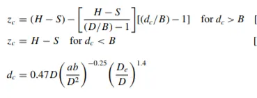
Iozia and Leith (1990) logistic model is a modified version of Barth (1956) model which is developed based on force balance. The model assumes that a particle carried by the vortex endures the influence of two forces: a centrifugal force, Z, and flow resistance, W. Core length, zc, and core diameter, dc are given as:
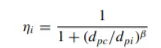
β is an expression for slope parameter derived based on the
statistical analysis of experimental data of a cyclone with D = 170
0.25 m given as:

and dpc is the 50% cut size given by Barth:
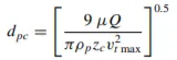
where core length, zc, and core diameter, dc, are given as
Model 2: Li and Wang Model
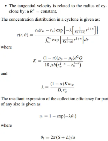
The Li and Wang [3] model includes particle bounce or re-entrainment and turbulent diffusion at the cyclone wall. A two-dimensional analytical expression of particle distribution in the cyclone is obtained. Li and Wang model was developed based on the following assumptions:
- The radial particle velocity and the radial concentration
- The profile is not constant for uncollected particles within the cyclone.
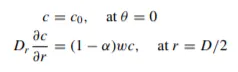
Boundary conditions with the consideration of turbulent diffusion coefficient and particle bounce entrainment on the cyclone wall are:
Model 3: Koch and Licht Model
Koch and Licht collection theory recognized the inherently turbulent nature of cyclones and the distribution of gas residence times within the cyclone. Koch and Licht described particle motion in the entry and collection regions with the additional following assumptions:
- The tangential velocity of a particle is equal to the tangential velocity of the gas flow, i.e. there is no slip in the tangential direction between the particle and the gas.
- The tangential velocity is related to the radius of the cyclone by u Rn = constant.
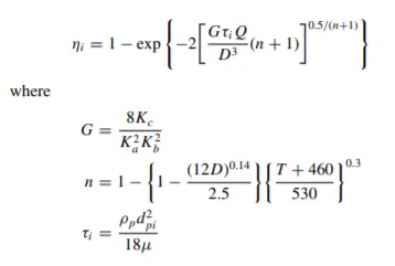
A force balance and an equation on the particles collection yields
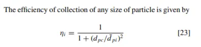
the grade efficiency ηi:
Model 4: Lapple Model
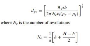
Lapple model was developed based on force balance without considering the flow resistance. Lapple assumed that a particle entering the cyclone is evenly distributed across the inlet opening. The particle that travels from inlet half-width to the wall in the cyclone is collected with 50% efficiency. The semi-empirical relationship developed by Lapple [1] to calculate a 50% cut diameter, dpc, is:
Solution Methodology :
This simulation is done using DPM .DPM is known as Discrete Phase Modeling .Usually DPM is employed when we want to represent one state of particles in another state of particles .That means if we want to represent solid particles in liquid particles or solid particles in gas particles. A discrete phase model (DPM) is used when the aim is to investigate the behavior of the particles from a Lagrangian view and a discrete perspective. In fact, the difference between the Lagrangian and the Eulerian view is that fluid behavior in Lagrangian view is examined on the basis of a particle tracking of a particle of fluid flow; Whereas fluid behavior is considered in Eulerian view based on the assumption of a finite volume element in the fluid flow path.
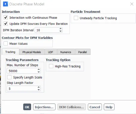
If the behavior of discrete particles in the presence of a continuous flow field is affected by continuous flow, the interaction with the continuous phase must be activated. Also, if the particle tracking is relatively unsteady over time, the unsteady particle tracking option must be activated. The discrete phase can be applied in various physical forms, the type of which depends on the problem model. One of the physical defining modes is the two-way turbulent coupling mode, which is used to study the effects of changes in the turbulent quantities caused by particle damping and Eddy turbulence. Also, the injection process for the mixed flow is defined in the input section of the model. In this way, in the input section of the model, the desired material enters the interior space of the model with the same discrete state or particle by particle. This particle injection as a discrete state can occur in different states. For example, the combusting mode is used when the material is injected into the model’s interior to perform the combustion process.
You can see some of the other projects can be used DPM model
- CFD simulation particle separator from gas using cyclone
- Using particle droplet combustion in two and four-stroke internal combustion engine
- Simulation particle settling by the gravity body force
- Wood combustion using the discrete phase model
- Sand particle tracking in the pond riverside
- Particle tracking in spray dryer using the DPM model
- Simulation of using magnetohydrodynamic (MHD) body force for increasing performance of cyclon
- errosion modeling in knee
Particle flow occurs in many engineering problems. For instance, some of its application areas in the industry are as follows. Fluidized beds, carbon capture, electrostatic reciprocator, solid separator cyclones, etc.. When investigating particle flow, we should take into account different phenomena. For example, the particles influence the overall properties of the fluid flow. They can change the heat transfer rate.
Moreover, different forces can affect particles. Forces such as electrical, electromagnetic and the forces between particles themselves. Designers of mechanical systems have an interest in predicting the trajectory of particles in the fluid flow. This is also very prominent when in the fluid flow charged particles and electromagnetic fields are present simultaneously.
ANSYS Fluent is a powerful CFD tool for the simulation of particle flows, and MR CFD Company is ready to organize your projects in this field.
Discrete Particle Behavior
Discrete particles have three different types of behavior in the presence of a continuous flow field:
Type 1) Discrete particles are not affected by the continuous phase.
Type 2) Discrete particles are affected by continuous flow (interaction with continuous phase).
Type 3) Discrete particles are affected by themselves, in addition to being affected by continuous phase (DEM collision).
Discrete Phase Boundary Condition
Discrete phases in boundary areas (such as inlet, outlet, and wall) can exhibit three different behaviors: ESCAPE, TRAP, and REFLECT. Usually, Escape condition is assumed in the inlets and outlets. While walls have Trap or Reflect conditions based on the problem description.
Particle flow is a kind of two-phase flow in which one phase is present continuously, usually named carrier phase. And the other phase (particle phase) consists of small immiscible particles in the fluid flow.
There are three approaches for modeling of particle-primary fluid interaction
- One way –this model just calculates the effect of primary fluid flow on particle path
- Two way –particle fluid flow and carrier fluid flow interact with each other simultaneously
- Four-way. Is like two way but also there is particle-particle interaction
SIMULATION :
Geometry :
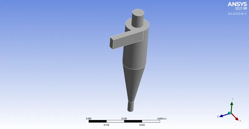
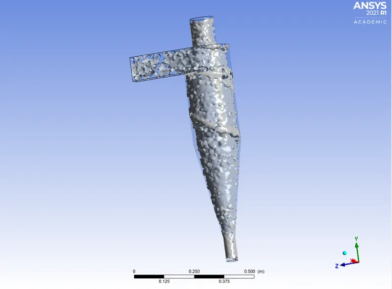
- Geometry of cyclone separator is impoerted in Ansys spaceclaim and the actual fluid volume is extracted using edge selection tool.
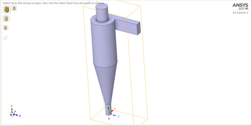
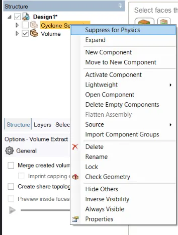
Unnecessary components are suppressed for physics.
Meshing :
- Extracted fluid volume from the actual cyclone separator geometry model is imported in Ansys meshing
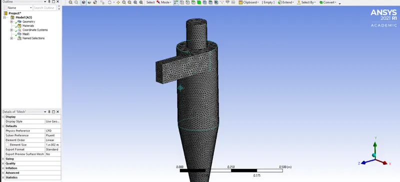
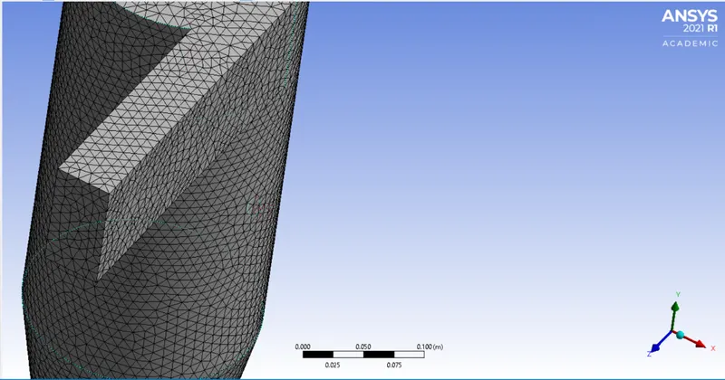
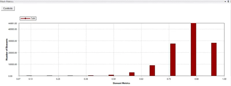
- First a base line mesh is generated and further it refined
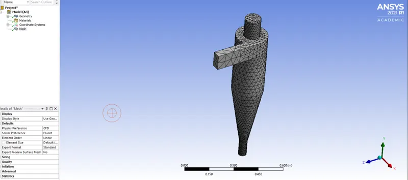
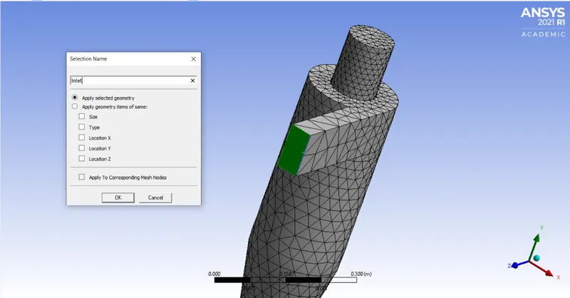
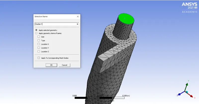
- Cyclone separator model has one inlet two outlet each at top and bottom as well .Those are named using named selection tool.
- Inlet:
- Outlet-1 (Top Outlet)
- Outlet 2(Bottom Outlet )
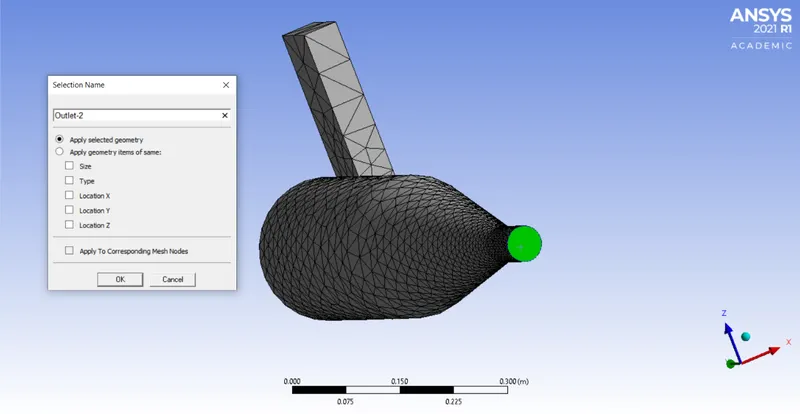
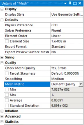
- Refined Mesh and its details :
PART 1 :
- Simulation is done in 2 parts for various differernt cases in order to analyse the cyclone simulator in Ansys Fluent .
- Geometry and meshing will be the same for those 2 parts .
- In this part 1 particle diameter varied from 1 Micro meter to 5 Micromter and for each diameter case , separation efficiancy calculated .Both flow velocity and particle velocity are taken as 3m/s.
Case-1
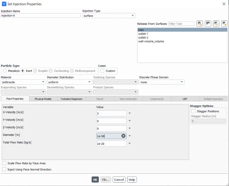
d= 1e-06m v= 3m/s
- Setup and solving :
-
Then the mesh model is now loaded in Fluent and necessary physics settings are set up. They are as mentioned below.
a) Solver : Pressure based steady state solver
b) Gravity : Enabled in -Y direction -9.81m/s^2
c) Viscous model : RNG k-epsilon with swirl dominant flow and standard wall functions
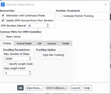
- DPM model detail
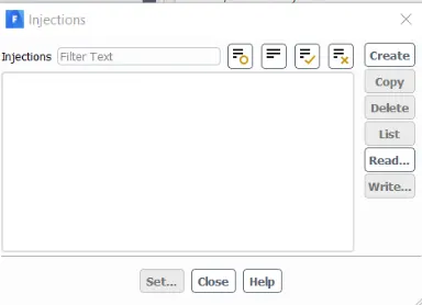
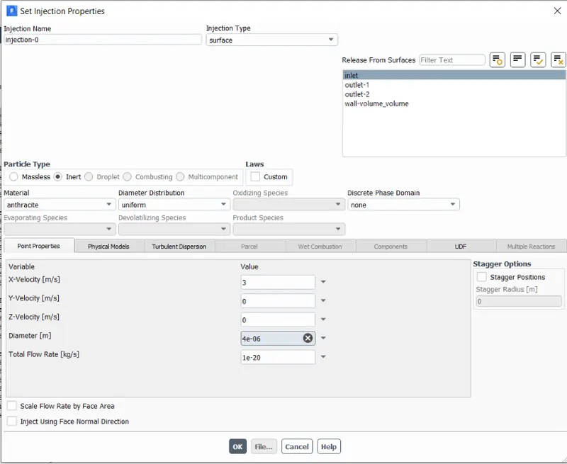
- Injections : Anthracite s
- Boundary Conditions:
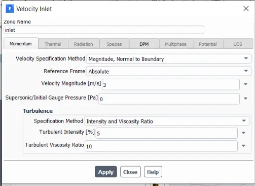
- Inlet :
Outlet 1 :
Outlet 2:
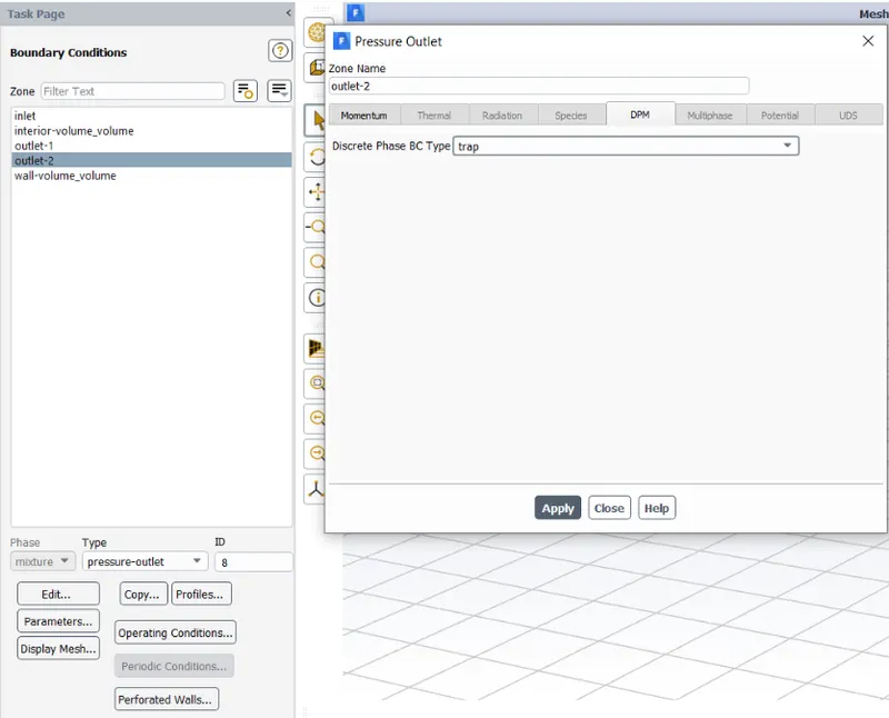
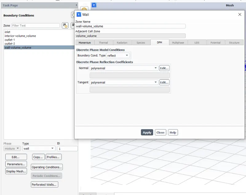
- The above boundary conditions are given in order to track the particles appropriately
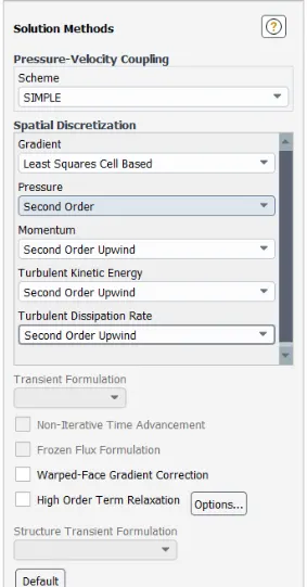
- Solution methods for this problem are able to capture these kind of flows perfectly
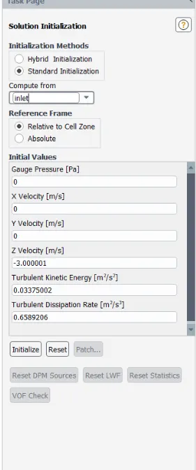
- Results :
- Residyuals :
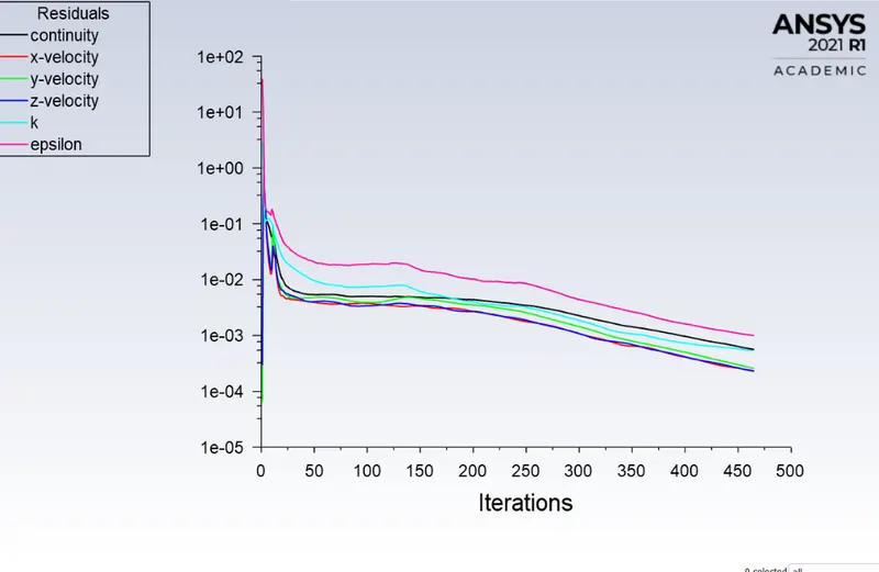

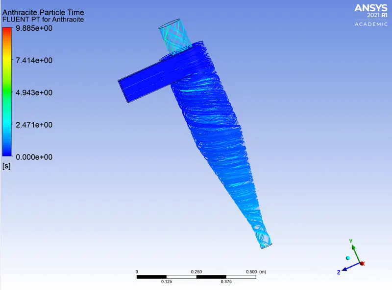
- 59 particles are incomplete this indicates that they were struck some where in the cyclone separator
- Separation Efficiency = (No. Of particles Trapped )/(No. Of Particles tracked )*100
- Case 1 Separation Efficiency =27.42%
- Particle Tracking and Post processing :
- Post processing has been done in CFD Post
- Particles path :
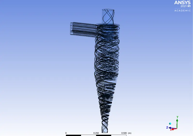
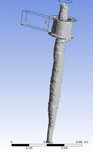
- Vortex core region
- Anthrecite particle time
- Animation :
- Case-2 ; d= 2e-06m v= 3m/s
- Details of particles

- Separation efficiency : 76.61%
- Particle injection
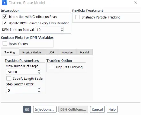
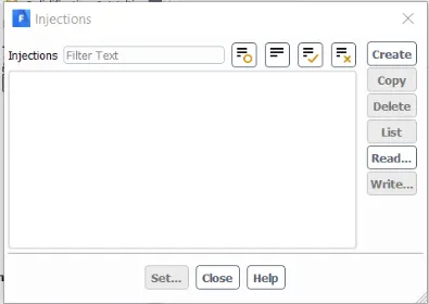
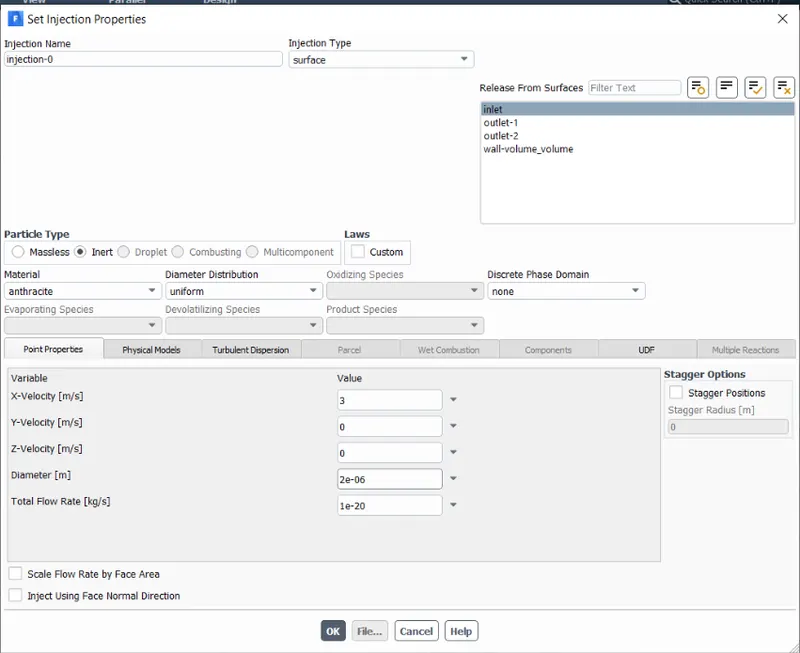
- Boundary conditions , solution methods and solution initialization is same as case 1
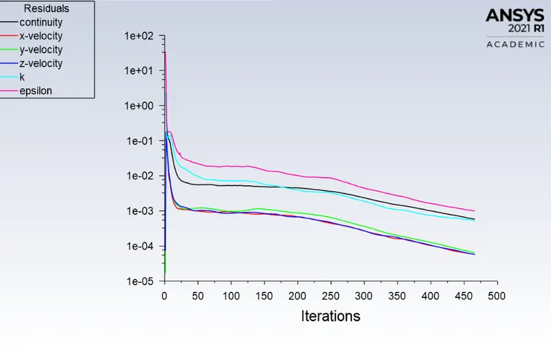
- Results :
- Residuals
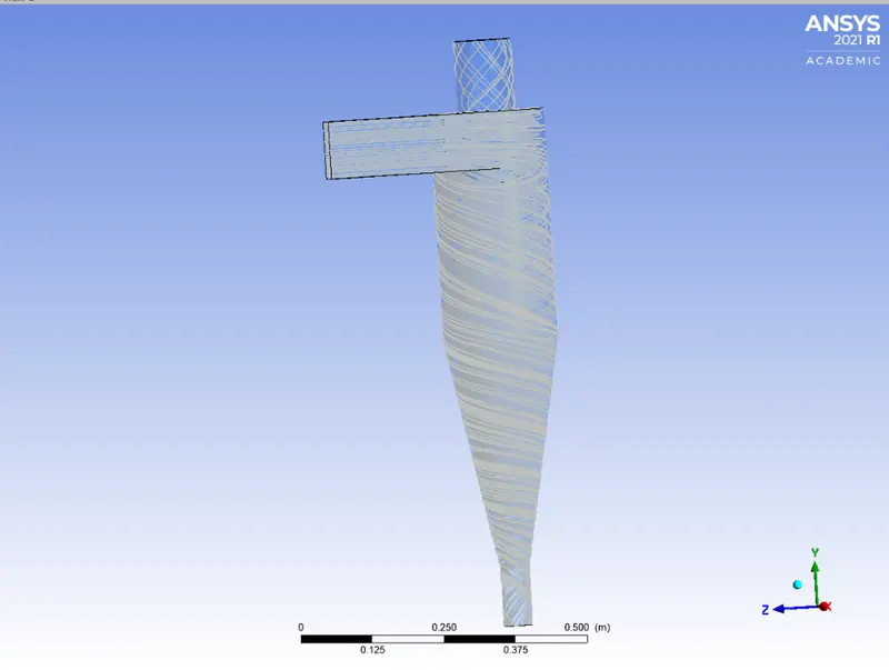
- Path of anthresite particles
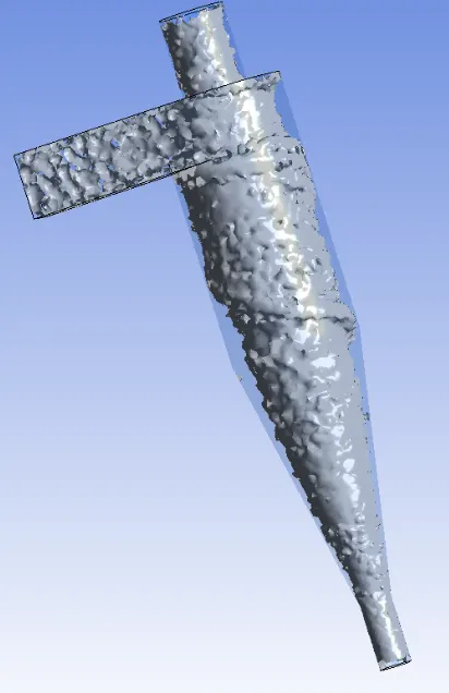
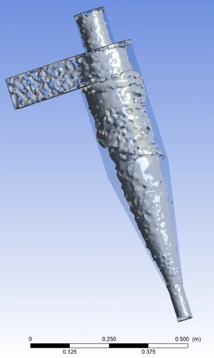
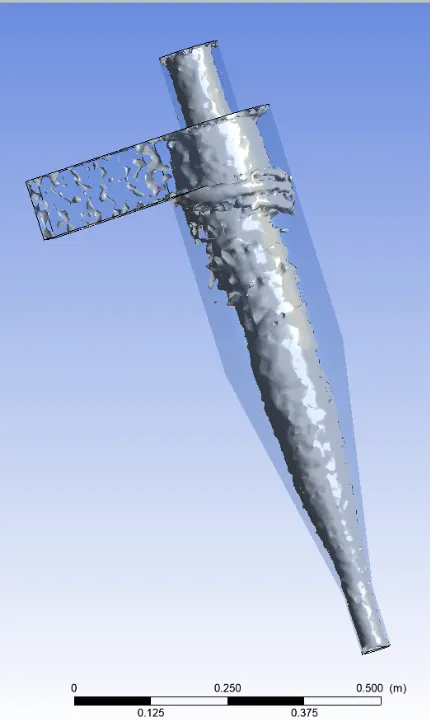
- Vortex core region at swirling strength 3.7761s^-1,9.59s^-1 and 23.25s^-1 respectively :
- Animation :
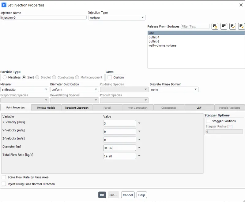
- Case-3 ; d= 3e-06m v= 3m/s
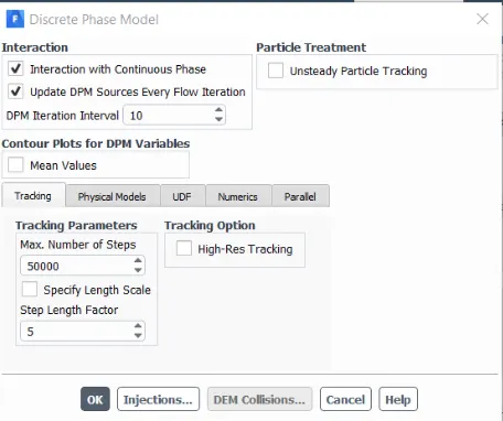
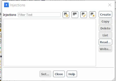
- DPM details
- Boundary conditions , solution methods and solution initialization is same as case 1
- Results :
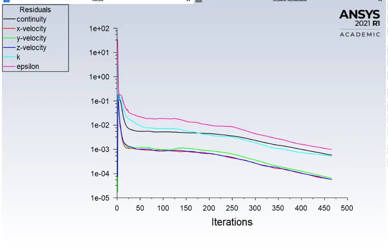
- Residuals :
- Details of particles

- Seperation Efficiency :82.23%
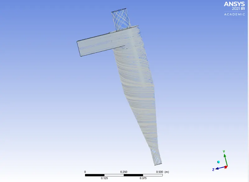
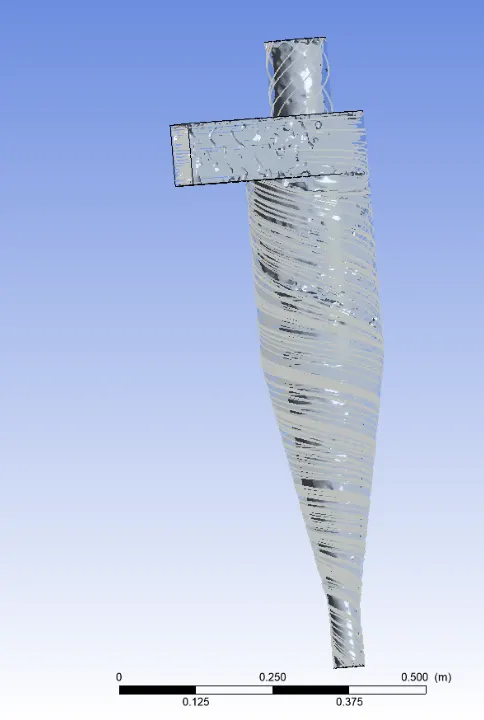
- Path of anthrecite partciles
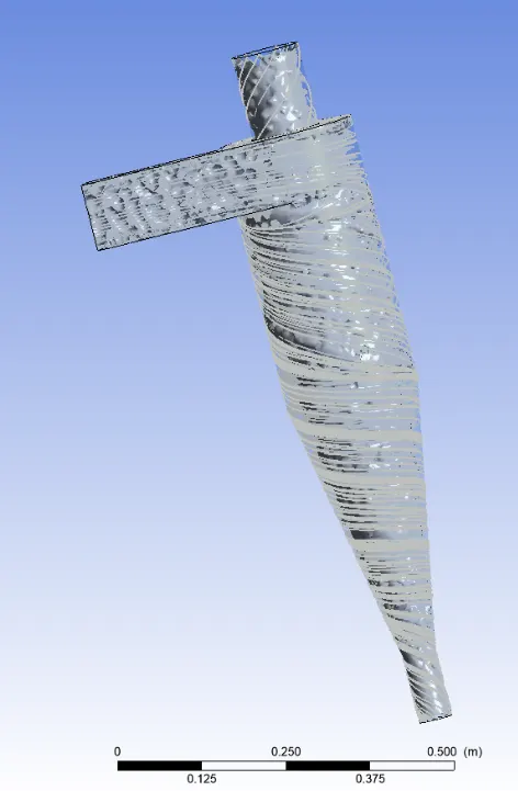
- Vortex region when swirling strength 3.77641s^-1 and 17.5505s^-1 respectively:
- Animation:
- Case-4 ; d= 4e-06m v= 3m/s
- DPM Details
- Details of particles :

- Separation efficiency = 88.71%
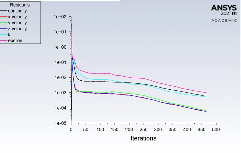
- Residuals
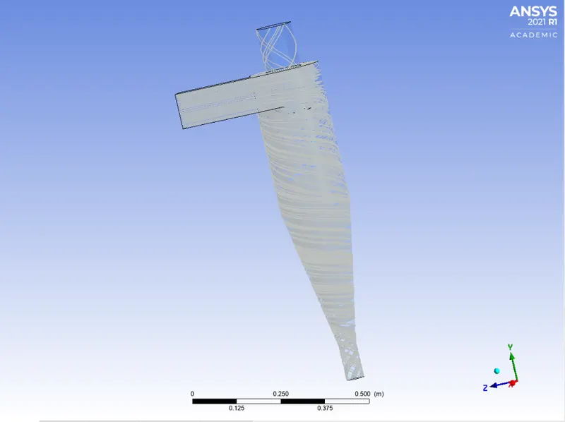
- Path of particles
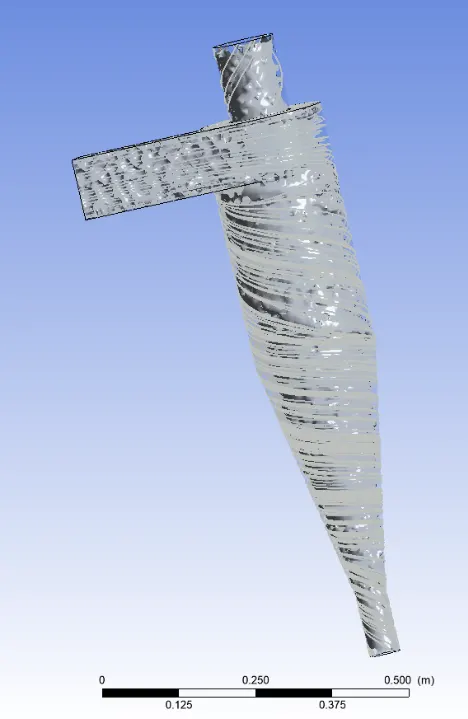
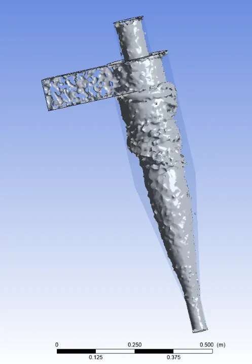
- Vortex core region at swirling strength 3.77s^-1 and 12.7982s^-1 respectively
- Animation :
Case-5 ; d= 5e-06m v= 3m/s
DPM details
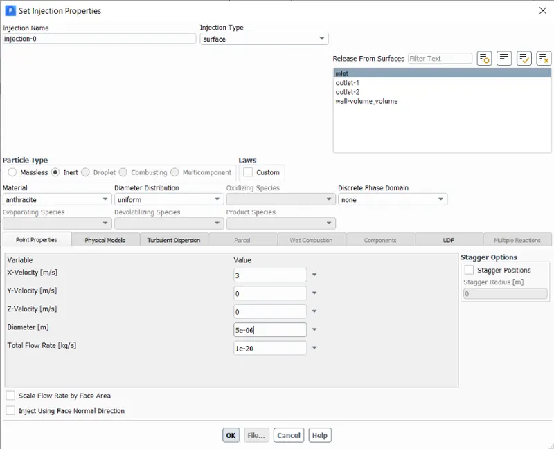
Details of particles :

Separation efficiency : 95.12%
Residuals
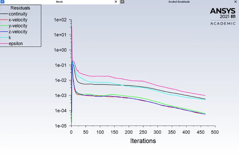
Path of particles
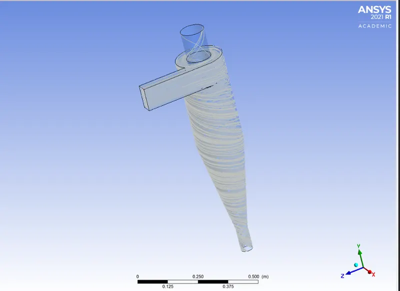
Vortex core region at swirling strength 13.643s^-1
Animation :
PART 2 :
- As mentioned earlier Simulation is done in 2 parts for various differernt cases in order to analyse the cyclone simulator in Ansys Fluent .
- Geometry and meshing will be the same for those 2 parts .
- In this part 2 particle velocity varied from 1m/s to 5 m/s and for each velocitycase , separation efficiancy, pressure drop calculated .Both flow velocity and particle velocity are taken as equal and particle diameter is 5micro meter
Case 1 : Particle Velocity 1m/s
- DPM settings
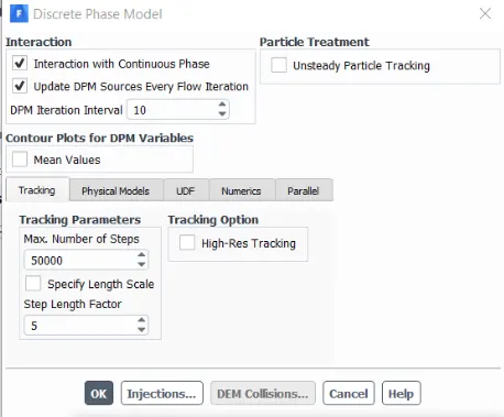
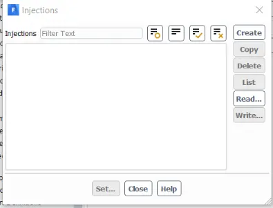
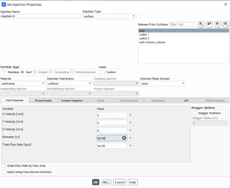
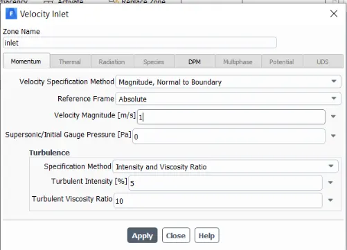
Boundary conditions
inlet :
solution methods
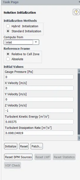
Results :
Particle details :

Separation Efficiency :0.097%
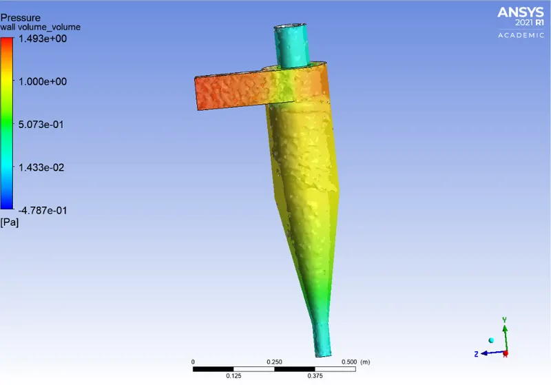
Contours od static pressure
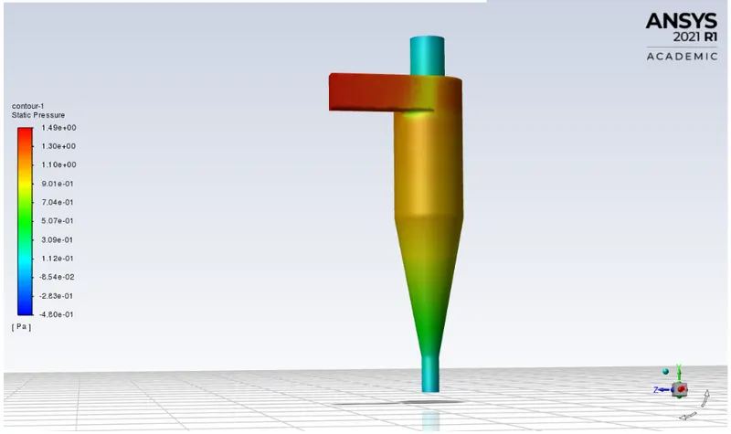
P_max = 1.49 Pa
P_min = -0.48 Pa
P_difference = 1.96Pa
- Residuals
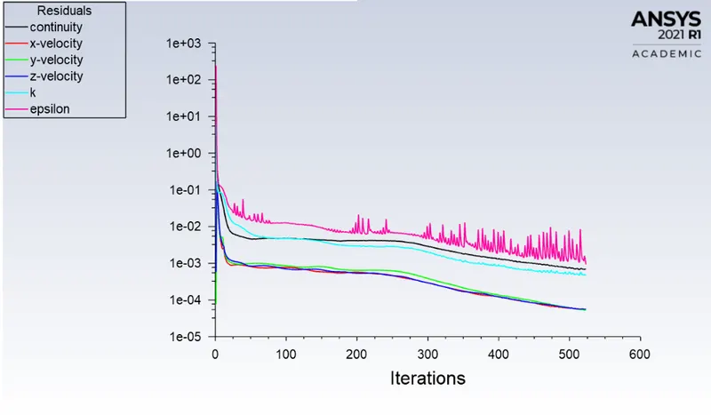
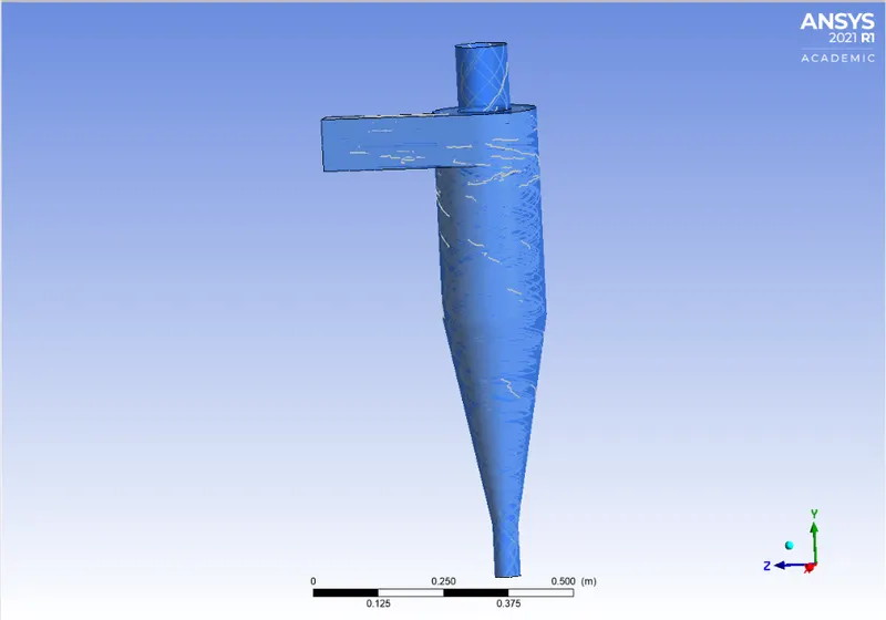
Path of anthrecite particles
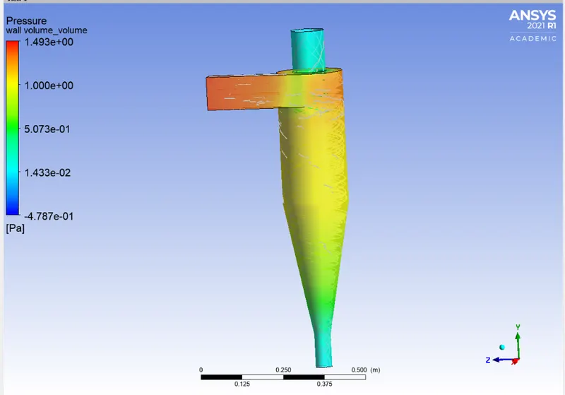
Pressure at wall
Anthrecite particle time :
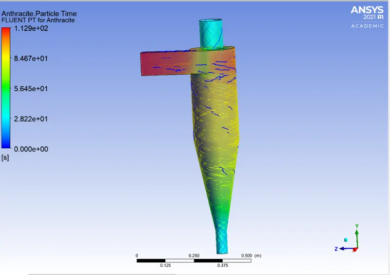
Vortex contour at swirling strength 3.132*91s^-1(@ pressure contour also) and at swrirling strength 3.13291 s^-1
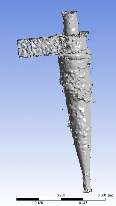
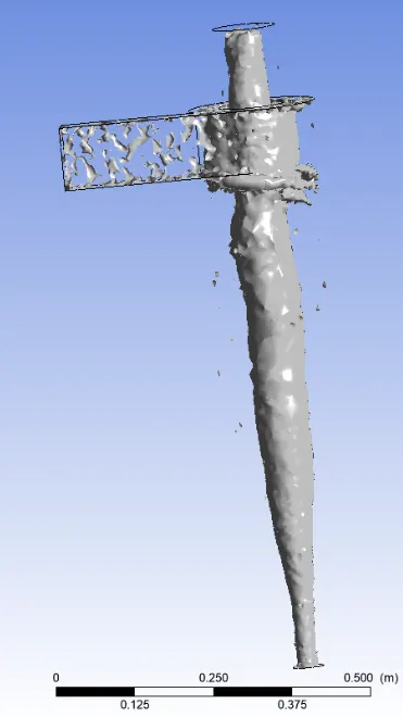
Animation
Case 2 : Particle Velocity 2m/s
- DPM Details :
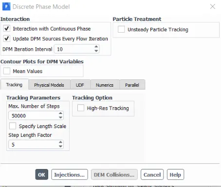
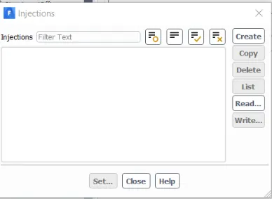
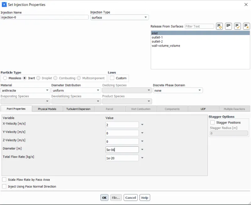
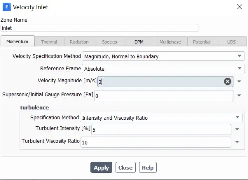
Inlet BC:
Solution and initialisation :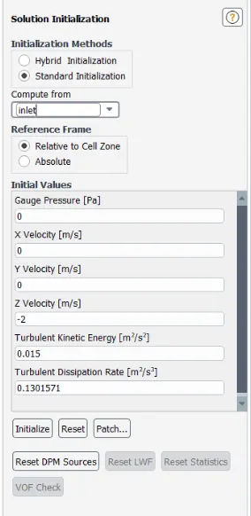
Results :
- Particle Details

Separation Efficiency : 0.08%
- Pressure Contour
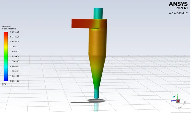
P_max = 6.66 Pa
P_min = -2.23Pa
P_difference = 8.89 Pa
- Residuals
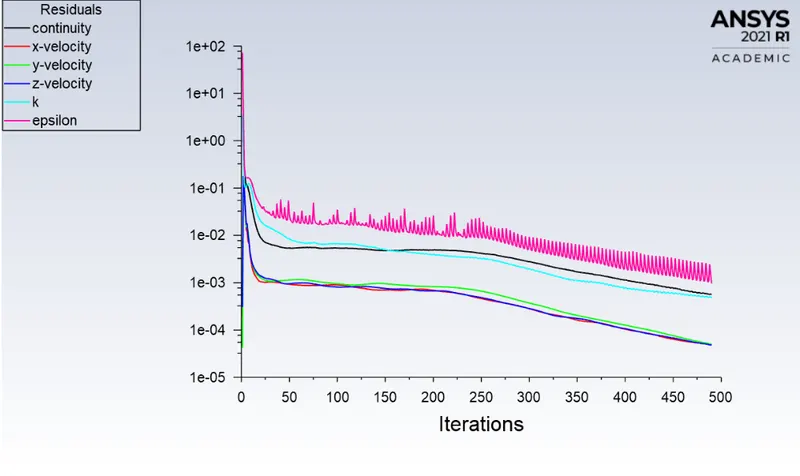
- Particle path
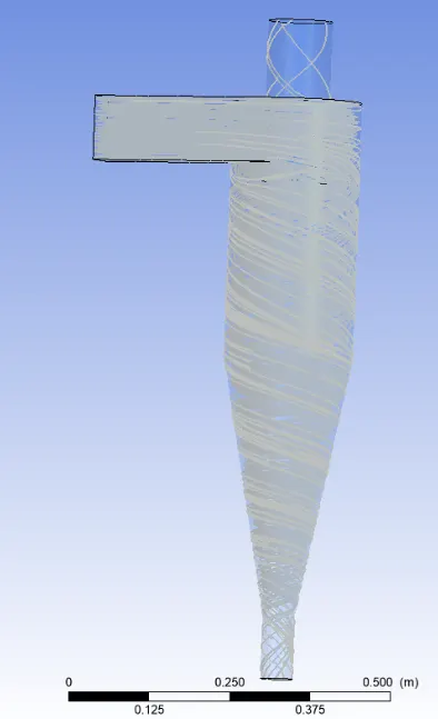
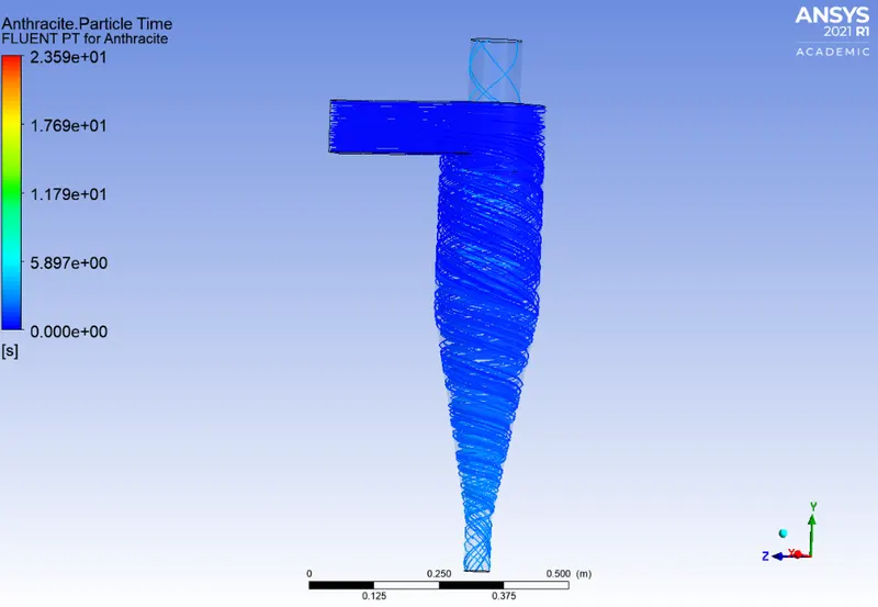
- Anthrecite Particle Time
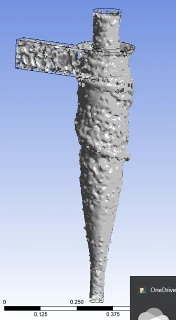
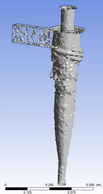
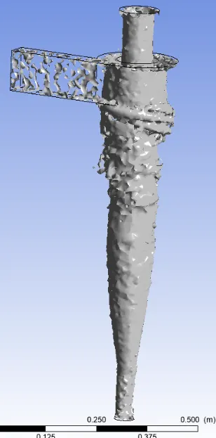
- Vortex core region at swrirling strength 1.8986s^-1, 12.6037s^-1 and
Animation :
Case 3 : Particle Velocity 3m/s
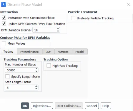
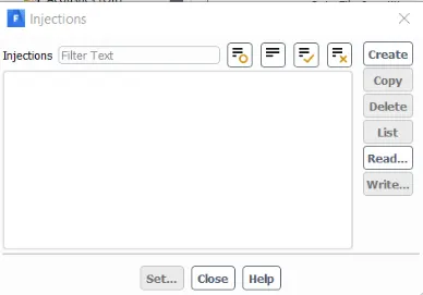
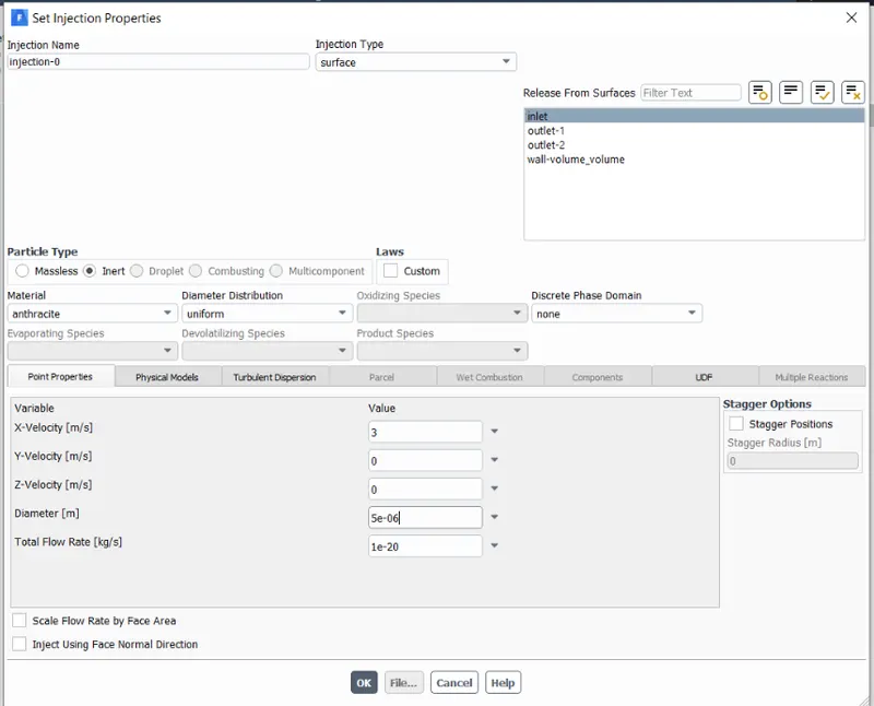
- DPM details
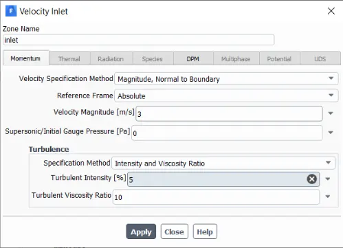
- Inlet Bc type
- Results
- Residuals
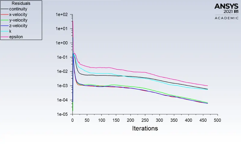
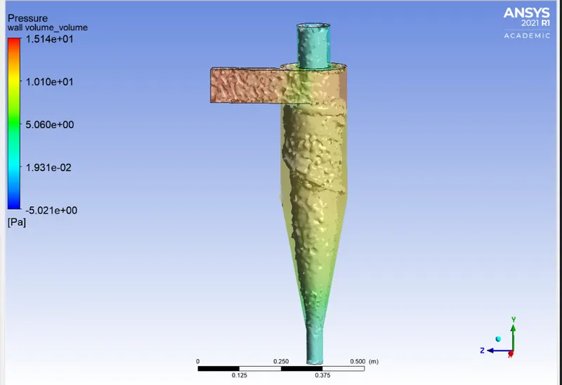
- Pressure details
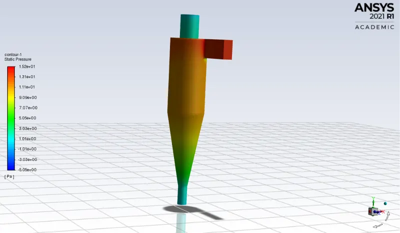
P_max = 15.2 Pa
P_min = -5.05 Pa
P_diffe = 2025 Pa
- Particle Tracking Details :

Separation Efficiency 95.12%
- Anthrecite Particle time
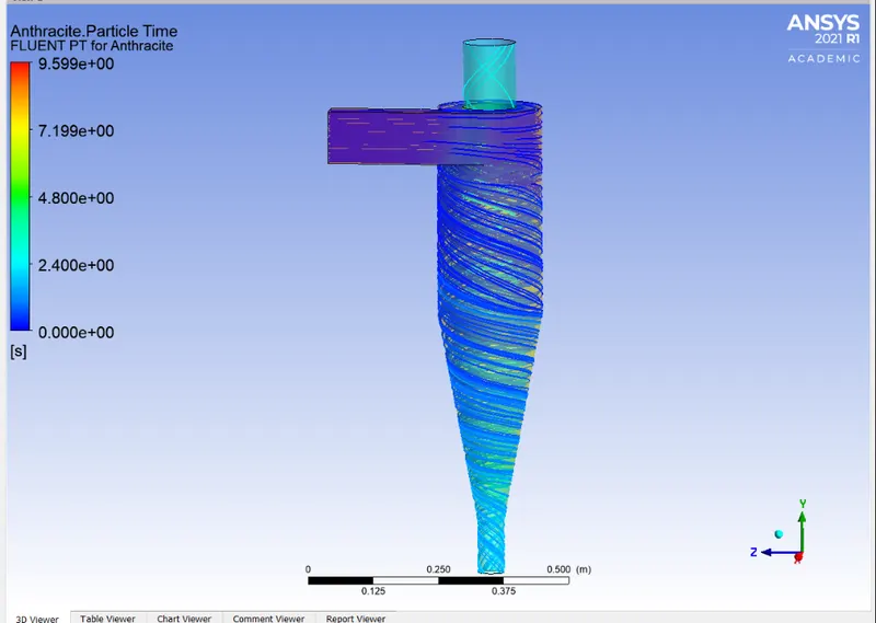
- Vortex core region at swirling strength 8.6641s^-1 along with pressure variation
- Animation :
Case 4 : Particle Velocity 4m/s
- DPM information
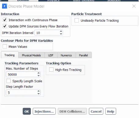
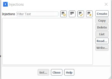
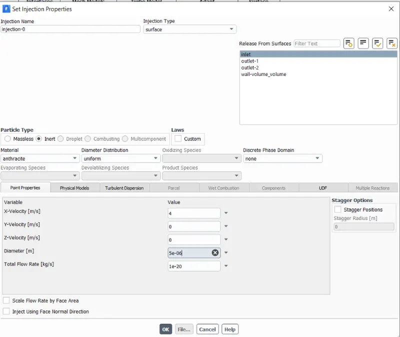
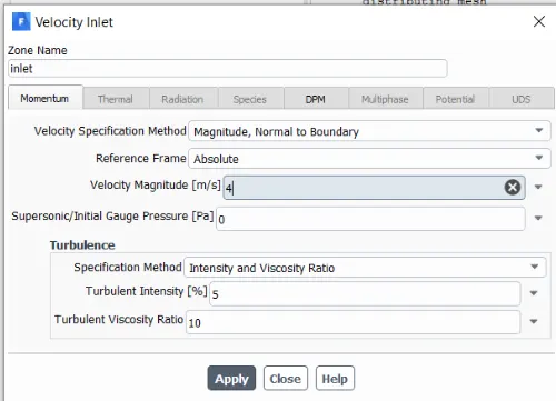
Inlet BC :
Solution Methods and initialiszation
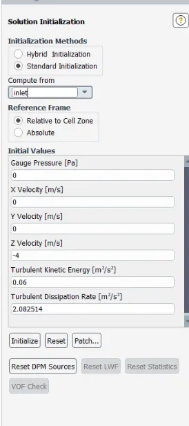
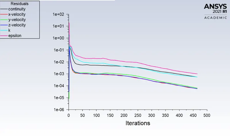
Results :
Residuals
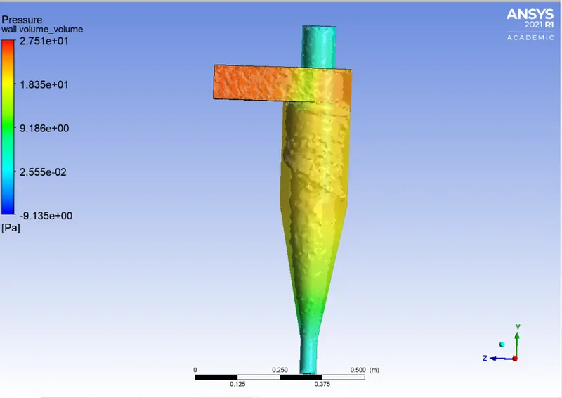
Pressure contour
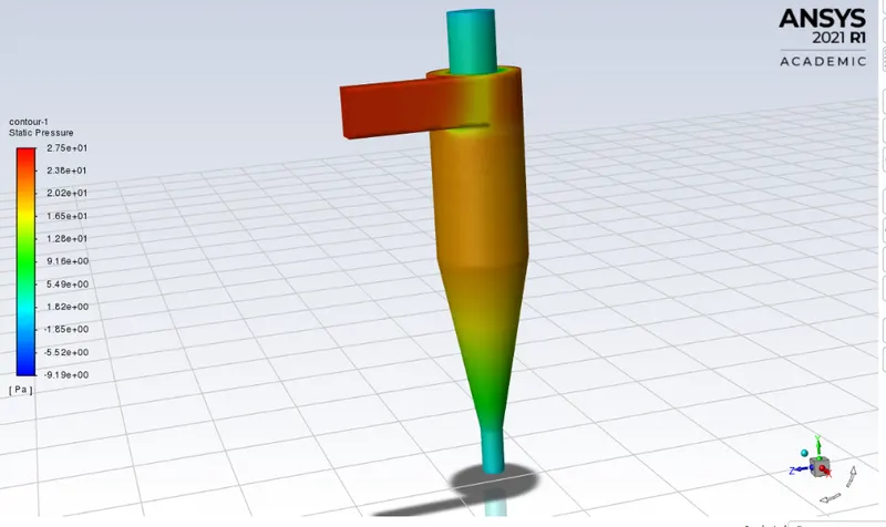
P_max = 27.5 Pa
P_min = -9.19 Pa
P_diff = 36.69 Pa
- Particle Tracking details

Separation efficiancy 98.34 %
- Particle path
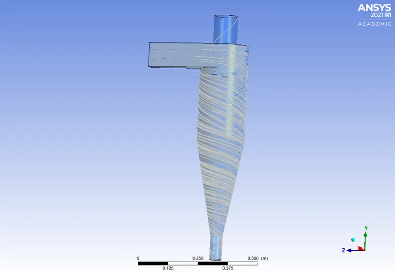
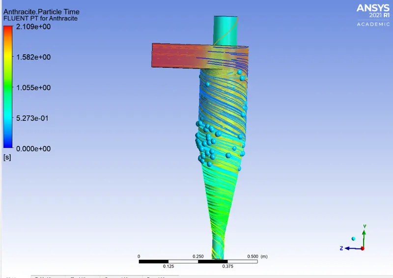
- Anthrecite particle tracking
- Vortex core region
- Animation :
Case 5 : Particle Velocity 5m/s
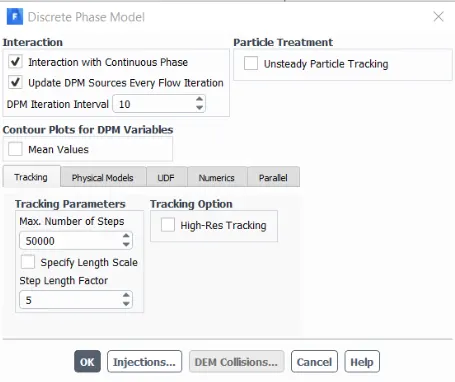
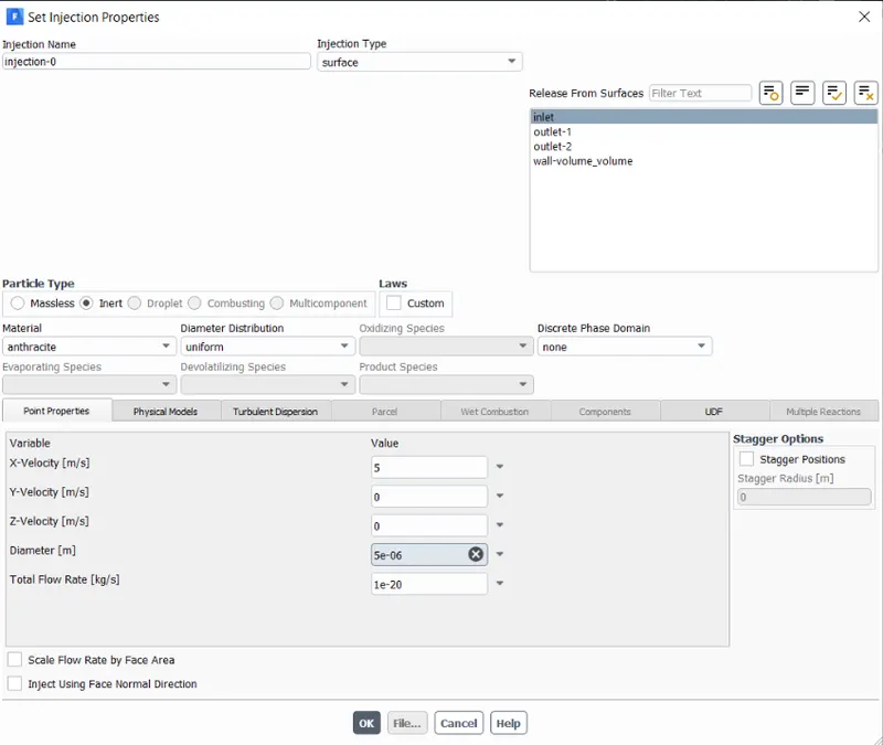
- DPM Details
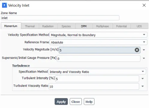
- Inlet Bc
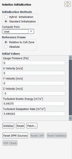
- Solution Initialization
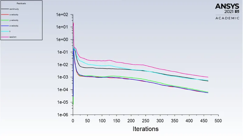
- RESIDUALS :
- Pressure Contour
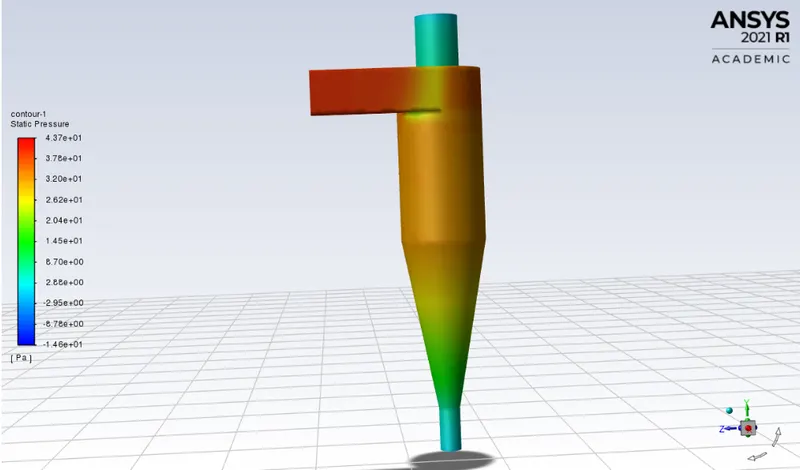
P_max = 43.7 Pa
P_min = -14.6 Pa
P_Diff = 58.3 Pa
- Particle tracking details :

Separation Efficiency 99.12%
- Paericle path :
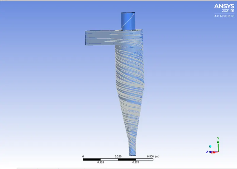
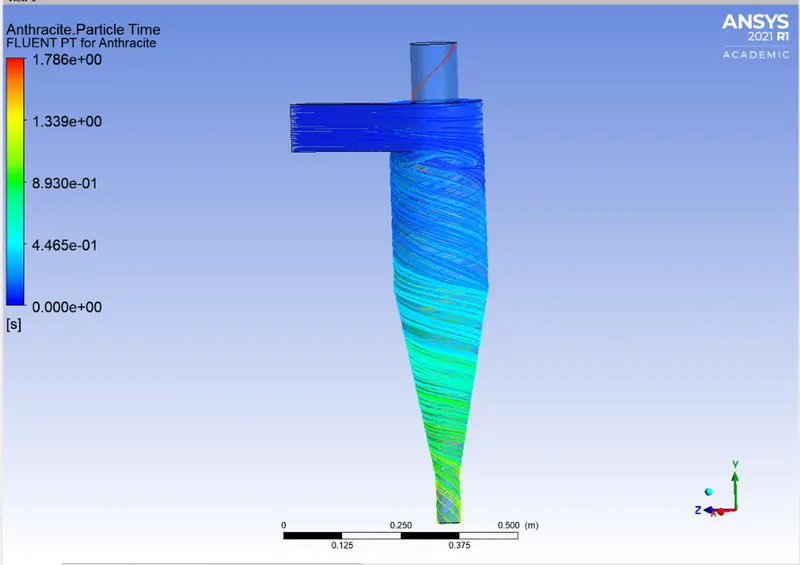
- Anthrecite particle time
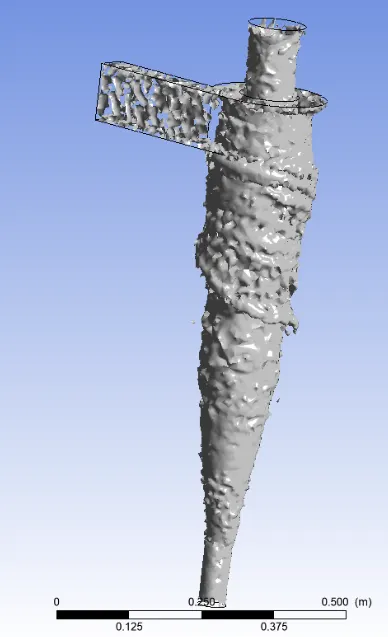
- Vortex core region at swirling strength 11.36s^-1 and 71.728s^-1 respectively
Animation :
PART 1 RESULTS COMPARISION :
| Case No. | Velocity Of Particle | Size Of Particle | Tracked | Trapped | Escaped | Incomplete | Separation Efficiency (%) |
| 1 | 3m/s | 1e-06m | 124 | 34 | 31 | 79 | 27.42 |
| 2 | 3m/s | 2e-06m | 124 | 95 | 27 | 2 | 76.61 |
| 3 | 3m/s | 3e-06m | 124 | 102 | 20 | 2 | 82.23 |
| 4 | 3m/s | 4e-06m | 124 | 110 | 13 | 1 | 88.71 |
| 5 | 3m/s | 5e-06m | 124 | 118 | 4 | 2 | 95.17 |
PART 2 RESULTS COMPARISION :
| Case No. | Velocity Of Particle | Size Of Particle | Tracked | Trapped | Escaped | Incomplete | Separation Efficiency (%) | Pressure Difference (Pa) |
| 1 | 1m/s | 5e-06m | 124 | 12 | 6 | 106 | 0.097 | 1.96 |
| 2 | 2m/s | 5e-06m | 124 | 10 | 5 | 100 | 0.08 | 8.89 |
| 3 | 3m/s | 5e-06m | 124 | 118 | 4 | 2 | 95.12 | 20.07 |
| 4 | 4m/s | 5e-06m | 124 | 122 | 2 | - | 98.34 | 36.69 |
| 5 | 5m/s | 5e-06m | 124 | 123 | 1 | - | 99.17 | 58.3 |
CONCLUSION
Based on the results discussed in the above , we can make the following conclusion:
- The efficiency of cyclone separators of the same size and configuration decreases as the particle size decreases.
- The efficiency of the cyclone separator s directly proportional to the flow velocity of the particulate. i.e. high-velocity yields higher efficiency
- Pressure drop only depends on the velocity of the particulate. As the velocity increases the pressure difference between inlet and outlet pressure increases.
- As the size of the particle decreases and the velocity of the flow decreases, the time is taken for convergence also increases. So to overcome this, the maximum no of steps in tracking parameters are increased.