Week 8 - Simulating Cyclone separator with Discrete Phase Modelling

Aim:- To perform analysis on cyclone separator and calculate the separation efficiency and pressure drop.

Objective:-

1. To write a few words about any four empirical models used to calculate the cyclone separator efficiency.
2. To perform an analysis on a given cyclone separator model by varying the particle diameter from 1 μm to 5 μm and calculate the separation efficiency in each case. Discuss the results. [Use both the velocity's as 3m/sec.]
3. To perform an analysis on a given cyclone separator model by varying the particle velocity from 1 m/sec to 5 m/sec and calculate the separation efficiency and pressure drop in each case. Discuss the results. [Use particle diameter size as 5 μm for all cases & keep flow velocity same as particle velocity]

Introduction

Cyclone separator: It is a device used for removing particulates from air, gas, or liquid stream, without the use of filters, through vortex separation. When removing particulate matter from the fluid a hydro cyclone is used, when removing particles from the gas a gas cyclone is used. Rotational effects and gravity are used to separate the mixture of solids and fluids.

Air is introduced into the cylinder exhibiting the vortex motion. The particulate matter having higher inertia do not follow the path prescribed by the air and thus hits the surface of the cyclone separator and falls at the bottom where it can be removed.

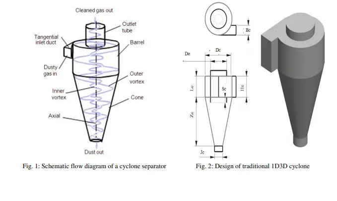
Application of cyclone separator

They are used in sawmills to remove sawdust from the extracted air. They are used in oil refineries to separate oils and gases, and in the cement industry as a component of kiln preheaters. They are also used as central vacuum cleaners in houses. They are also used in industrial and professional kitchen ventilation for separating the grease from the exhaust air in extraction hoods.

Empirical models used to calculate the cyclone separator efficiency

Cyclone Efficiency Empirical Models

IOZIA and LEITH model

The above model is the modified logistic model of Barth. The model assumes that the particle carried by the vortex endures the influence of two forces: a centrifugal force Z, and a flow resistance W, Core length,z, and core diameter, `d_c` are given as

Equation 1(a)

for `d_c>B`

`z_c=(H-S)-[frac{H-S}{(D/B)-1}][(frac{d_c}{B})-1]`

Equation 1(b)

for `d_c<B`

`z_c=H-S`

Equation 2

`d_c=0.47[frac{ab}{D^2}]^-0.25**[frac{D_e}{D}]^1.4`

The addition made by the two scientists with respect to the Barth was core length `z_c` and the slope parameter `beta`. The collector efficiency on a particle diameter `d_(p i)` for the cone diameter `D=0.25m`

Equation 3

`eta_i=frac{1}{1+(frac{d_(pc)}{d_(p i)^-})^beta`

Equation 4

`d_(pc)` is the `50%` cut size given by Barth in 1956.

where `d_(pc)=[frac{9muQ}{piP_pz_cv_(max)^2}]^0.5`

LI and WANG model

The above model includes particle bounce, re-entrainment, and turbulent diffusion at the cyclone wall. The model was developed on the following assumptions

• The radial velocity and the radial concentration profile are not constant for the uncollected particle.
• The boundary condition with the consideration of turbulent diffusion coefficient and particle bounce re-entrainment on the cyclone wall is given as

Equation 5

`c=c_0`, `theta=0`

Equation 6

`D_rfrac{delc}{delr}=(1-alpha)wc`, at `r=frac{D}{2}`

The tangential velocity is related to the cyclone wall by `uR^n` `=` constant.

The concentration distribution in a cyclone is given as

Equation 7

`c(r,theta)=frac{c_0(r_w-r_n)exp{-lambda[frac{1}{K(1+n)}r^(1+n)]}}{int_(r_n)^(r_w)exp{frac{1}{K(1+n)}r^(1+n)}dr}`

Equation 8

where

`k=frac{(1-n)(rho_p-rho_g)d^2Q}{18mub(r_w^(1-n)-r_n^(1-n))}`

Equation 9

`lambda=frac{(1-alpha)kw_w}{D_rr_w^n}`

The resultant expression of the collector efficiency of the particle is given as

Equation 10

`eta=1-exp{-lambdatheta_1}`

Equation 11

where

`theta_1=2pifrac{(S+L)}{alpha}`

KOCH and LICHT model

The model recognized the inherently turbulent nature of cyclones and the distribution of gas residence times within the cyclone. The model is based on the following assumption

• The tangential velocity of the particle is equal to the tangential velocity of the gas flow and there is no slip condition involved in the tangential direction between the particle and the gas.
• The tangential velocity is related to the radius of the cyclone by `uR^n=` constant.

The grade efficiency of the particle is calculated as under

Equation 12

`eta_i=1-exp{-2[frac{Gtau_iQ}{D^3}(n+1)]^frac{0.5}{n+1}}`

Equation 13

`G=frac{8k_c}{k_a^2k_b^2}`

Equation 14

`n=1-{1-frac{(12D)^0.14}{2.5}}{frac{T+460}{530}}^0.3`

Equation 15

`tau_i=frac{rho_pd_(p i)^2}{18mu}`

G is a factor related to the configuration of the cyclone, n is related to the vortex and `tau` is the relaxation term.

LAPPLE Model

Lapple assumed that the particle entering the cyclone is evenly distributed across the inlet opening. The particle that travels inlet half-width to the wall in the cyclone is collected with `50%` efficiency. The semi-empirical relationship developed by Lapple to calculate a `50%` cut diameter, `d_(pc)`, is

Equation 16

`d_(pc)=[frac{9mub}{2piN_ev_i(rho_p-rho_g)}]^frac{1}{2}`

Equation 17

where `N_e` is the number of revolutions

`N_e=frac{1}{a}[h+frac{H-h}{2}]`

Equation 18

The efficiency of the particle collection is given as

`eta_i=frac{1}{1+(frac{d_(pc)}{d_(p i}^-})^2`

Source: http://dspace.unimap.edu.my

Solving and Modeling approach

• The geometry is loaded into Spaceclaim.
• The fluid volume is extracted from the solid volume.
• The solid volume is suppressed for physics.
• The geometry is loaded into meshing.
• The named selections are created for the required geometry (inlet, outlet_top,outlet_bottom).
• It is then discretized into various cells, first, the simulation is run for the baseline mesh, by keeping the velocity `3msec^-1` as constant and changing the particle size from `1mum` to `5mum`.
• After the results have been executed properly for the baseline mesh, the mesh refinement approach is followed by varying the parameters.
• The setup is done for the required geometry, setting up the viscous model, discrete phase modelling is selected for the same.
• The necessary contour images have been uploaded for the same.
• The efficiency of the cyclone separator is calculated for each case.
• The conclusion and references are drawn from the tabulated data.

Preprocessing and Solver settings

The geometry is loaded into Spaceclaim

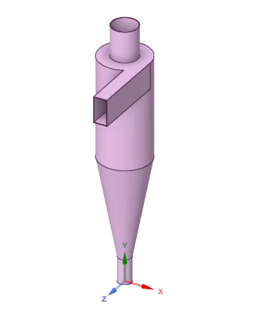
The fluid volume is extracted from the solid volume

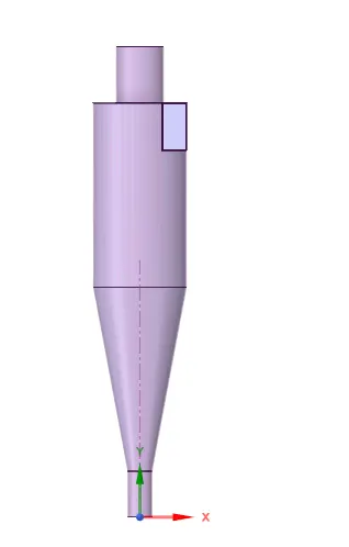
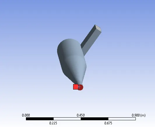
The named selections are created for setting up the physics and the boundary condition

Inlet (Type Velocity inlet and Reflect)

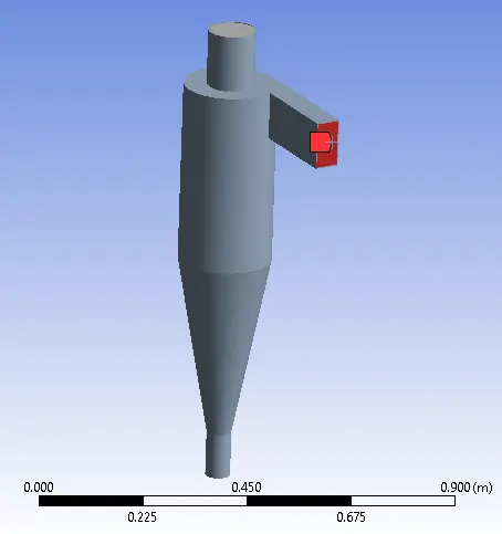
Outlet_top (Type Pressure outlet and Escape)

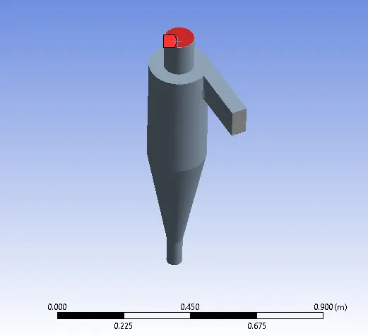
Outlet_bottom (Type Pressure outlet and Trap)

Baseline mesh

Element size: 55.916mm

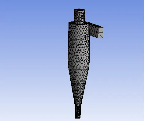
Mesh quality and attributes

Number of elements	Element quality	Aspect ratio	Skewness	Orthogonal quality
`20370`	`0.8201`	`1.9581`	`0.25021`	`0.74779`

Refined mesh

Element size : 10mm

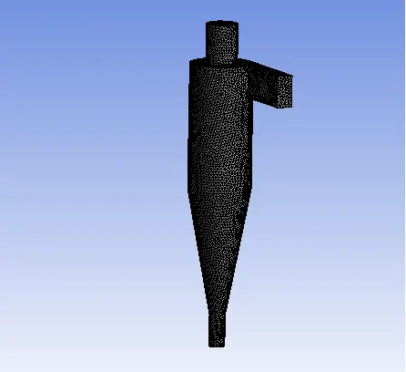
Mesh quality and attributes

Number of elements	Element quality	Aspect ratio	Skewness	Orthogonal quality
`112565`	`0.83691`	`1.8571`	`0.22862`	`0.76952`

Element size: 9mm

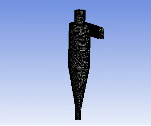
Mesh quality and attributes

Number of elements	Element quality	Aspect ratio	Skewness	Orthogonal quality
`141918`	`0.83836`	`1.8508`	`0.22633`	`0.7718`

Element size : 8mm

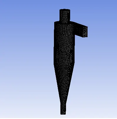
Mesh quality and attributes

Number of elements	Element quality	Aspect ratio	Skewness	Orthogonal quality
`185349`	`0.83779`	`1.8513`	`0.22746`	`0.77072`

Set up

• The steady-state pressure-based solver is selected (`Mlt0.3`).
• The gravity option is enabled and `-9.81msec^-2` is enabled for the y-axis.
• The energy option is not required for the cyclone separator simulation therefore it is disabled.

Turbulence model RNG `k-epsilon`

• The viscous model is set to `k-epsilon``RNG` swirl dominated flow is selected for accuracy. The `k-epsilon` turbulent model consists of two transport equation turbulent kinetic energy (K) and turbulent dissipation epsilon (`epsilon`) to calculate the rate of dissipation of turbulent kinetic energy K. In this particular simulation the model being used is RNG `k-epsilon` model. The difference between RNG `k-epsilon` and the standard `k-epsilon` model are as follows.
• It is used for swirling flows.
• Additional terms used in `epsilon`is used for improving the accuracy of the solution
• Near wall treatment as Standard wall function is selected.

Setting up of boundary condition

• Inlet (type velocity inlet and reflect): The velocity inlet is varied from `1msec^-1` to `5msec^-1` and the discrete phase modelling condition is set to reflect.
• Outlet_top (type pressure outlet and escape): The gauge pressure is set to 0Pa, and the discrete phase modelling is set to escape.
• Outlet_bottom (type pressure outlet and trap): The gauge pressure is set to 0Pa, and the discrete phase modelling is set to trap.
• Wall (type no-slip and reflect): The boundary condition for the wall is no-slip(shear condition) and the wall condition is stationary and discrete phase modelling is set to reflect.

Setting up of Discrete Phase Modelling

The discrete phase modelling consists of the dispersed phase and the fluid phase. The behaviour of the fluid phase (air) is being captured by the NS equation whereas the tracking of the dispersed phase (anthracite) is solved by tracking a large number of droplets, particles through the calculated flow field. The dispersed phase exchanges the momentum, mass flow rate, and energy within the fluid phase.

There are two types of coupling for the discrete phase modelling

• The fluid interacts with the dispersed phase via drag and turbulence, but the dispersed phase does not interact with the fluid. This is called one-way coupling.
• The fluid interacts with the dispersed phase via drag and turbulence, and the dispersed phase transfers mass, momentum, and energy. This is called two-way coupling.

The DPM is selected from the ribbon

The interaction with the continuous phase is selected as such it will be a coupled interaction the dispersed phase will transfer momentum to the fluid phase. The update DPM after every flow iteration is checked so that it calculates the source term of each particle so that the particles reaches their constant value, whereas the default values are retained for Max. number of steps, DPM iteration level, step length factor which is 50000 10 & 5 respectively. The particle size is varied accordingly to determine the efficiency of the cyclone separator.

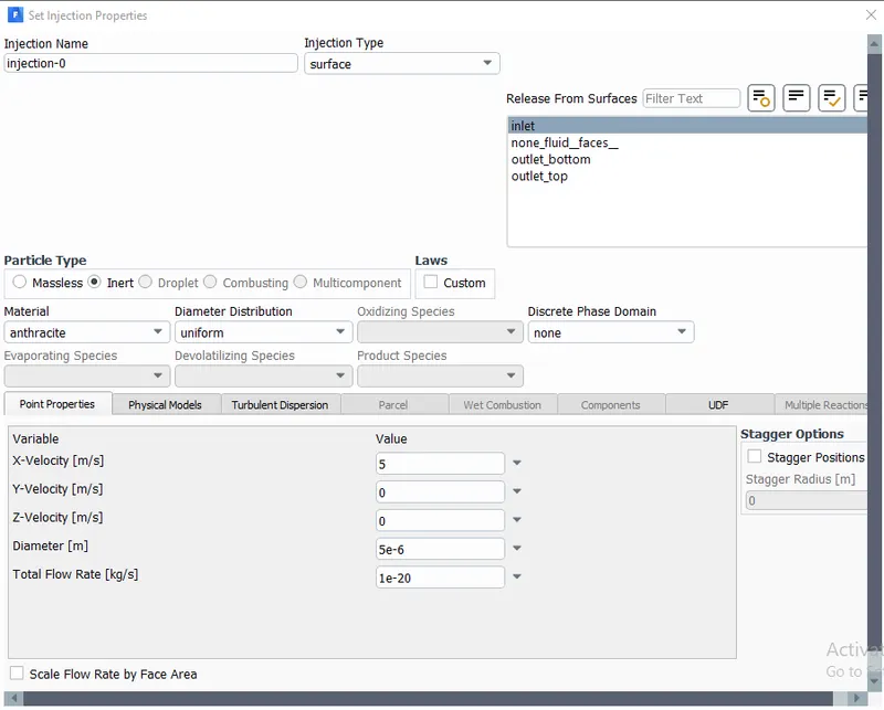
The solution is standard initialized by hitting `t=0` and the compute from inlet option is selected.

Case-1

Baseline mesh

Pressure-Velocity coupling schemes (SIMPLE)

Residual Plot

Inlet velocity `3msec^-1`

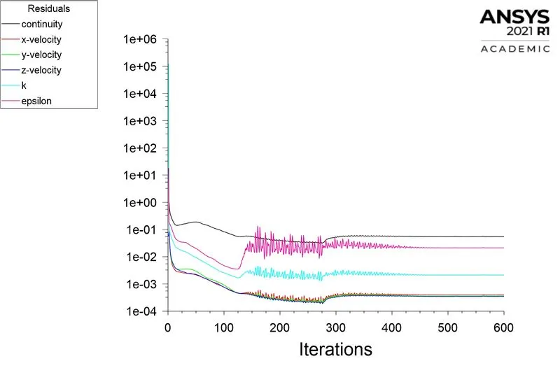
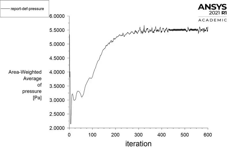
Area weighted average of pressure

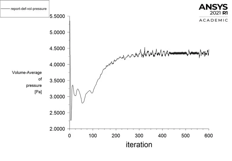
Volume average of pressure

Pressure-Velocity coupling schemes (SIMPLEC)

Inlet velocity `3msec^-1`

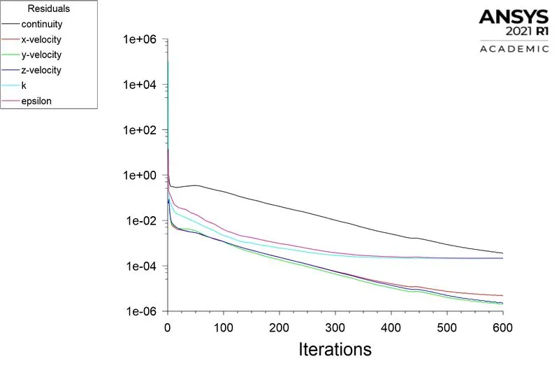
Residual Plot

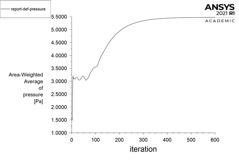
Area weighted average of pressure

Volume average of pressure

Pressure-Velocity coupling schemes (COUPLED)

Inlet velocity `3msec^-1`

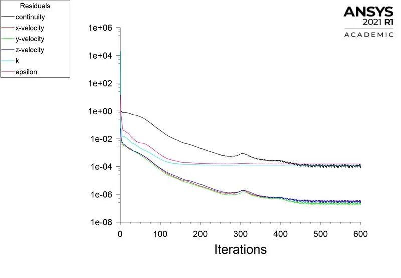
Residual plot

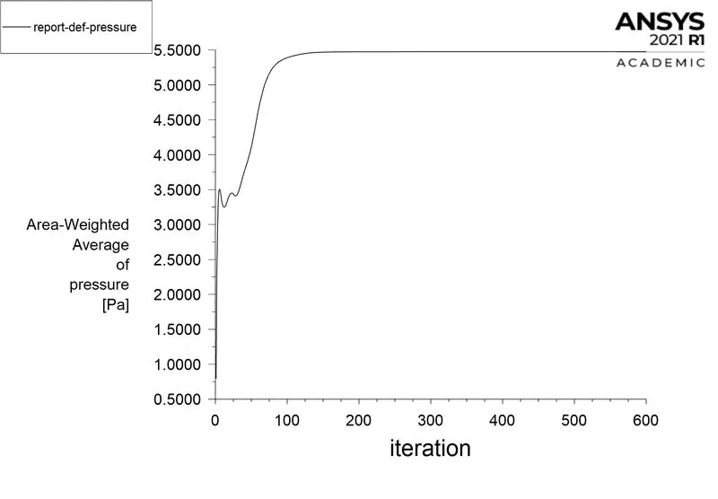
Area weighted average of pressure

Volume average of pressure

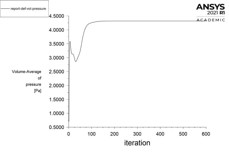
Mesh	Element size	Number of elements	Pressure-velocity coupling scheme	Area weighted average of pressure (Pa)	Volume average of pressure (Pa)
Baseline mesh	55.916mm	`20370`	SIMPLE	`5.6146`	`4.4622`
			SIMPLEC	`5.4714`	`4.3152`
			COUPLED	`5.4741`	`4.3171`

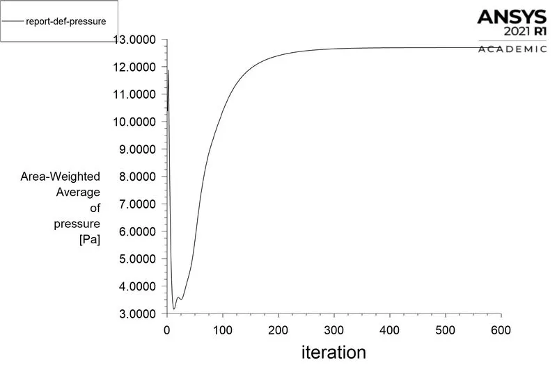
It can be inferred that the baseline mesh is run by using a particle size of 5e-6 m and the particle velocity having the value of 3 m/sec by using three different pressure-velocity coupling schemes (SIMPLE, SIMPLEC, COUPLED). It was observed that the most stable values of pressure were given by the COUPLED SCHEMES. It also takes less time for convergence because the pressure and velocity equations are solved instantaneously. It takes more space from segregated schemes (SIMPLE and SIMPLEC).The monitor plots for the COUPLED scheme took 100 iterations for convergence and after that it reaches to the steady-state, for the SIMPLEC scheme it took around 300 iterations for convergence and after that it reaches to the steady-state, for the SIMPLE scheme the graph is oscillating in nature.

For the COUPLED scheme, the gradient is selected as least square cell-based, pressure to the second-order scheme, momentum, turbulent kinetic energy, turbulent dissipation rate to second-order upwind. The least cell-based values are used to calculate the change in the value of the centroid of the two cells and offering comparable accuracy and is computationally less expensive to the node-based scheme. The second order scheme uses a central differencing scheme which is more accurate than standard and linear based schemes and is robust in the case of skewed schemes. Second-order upwind schemes make use of quantities at the cell face values to compute the cell centered solution of the at the cell centroid leading to a second order accurate solution.

Results

The particle size is varied from `1e-6m` to `5e-6m` keeping the velocity as `3msec^-1` and accordingly cyclone separator efficiency is calculated for each case.

Case-2 Refined mesh

Element size: `10mm`

Number of elements: `112565`

Particle size: `1e-6m`

Inlet velocity: `3msec^-1`

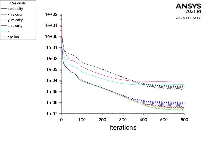
Residual Plot

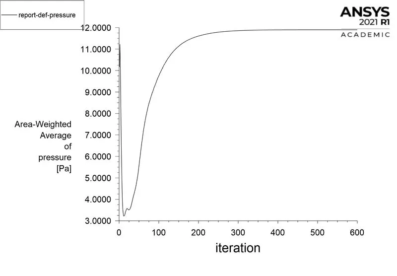
Area weighted average of Pressure

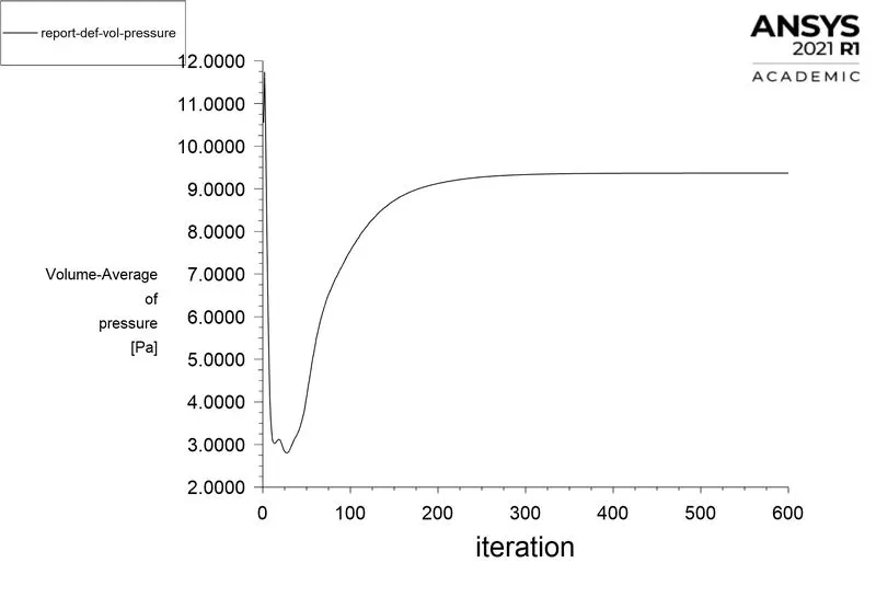
Volume average of Pressure

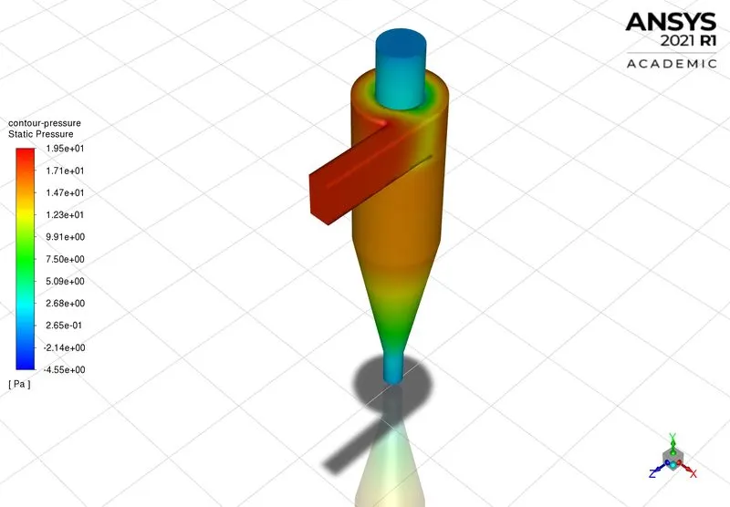
Static Pressure

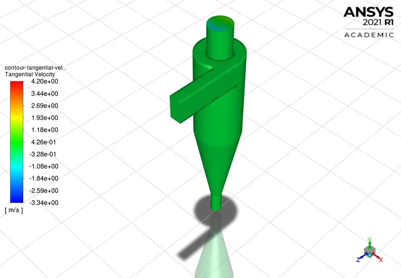
Tangential Velocity

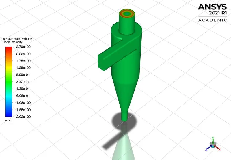
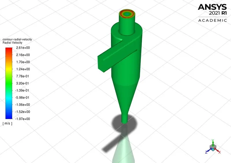
Radial Velocity

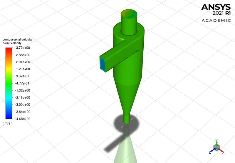
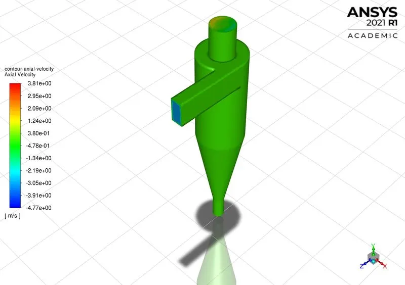
Axial Velocity

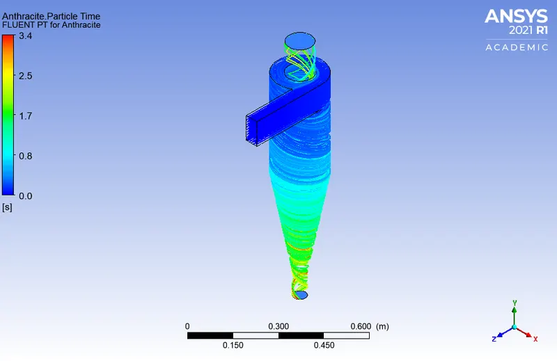
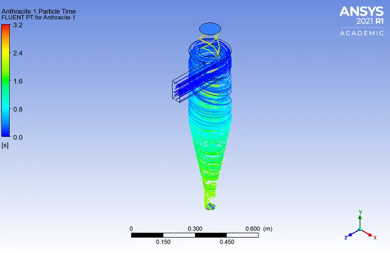
Anthracite Particle Time

Element size: `9mm`

Number of elements: `141918`

Particle size: `3e-6m`

Inlet velocity: `3msec^-1`

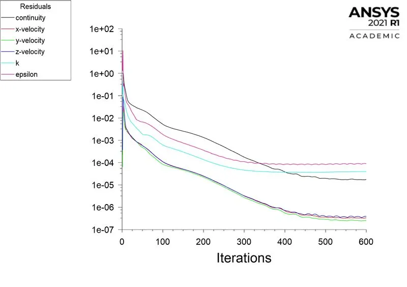
Residual Plot

Area weighted average of Pressure

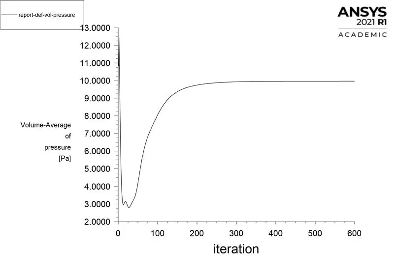
Volume average of Pressure

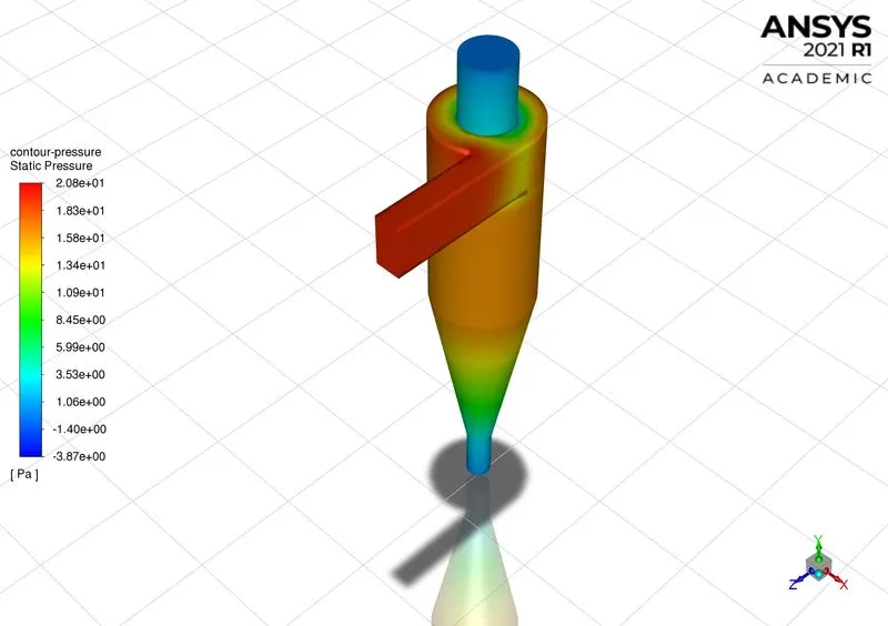
Static Pressure

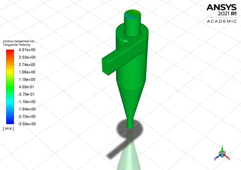
Tangential Velocity

Radial Velocity

Axial Velocity

Anthracite Particle Time

Element size: `8mm`

Number of elements: 185349`

Particle size: `5e-6m`

Inlet velocity: `3msec^-1`

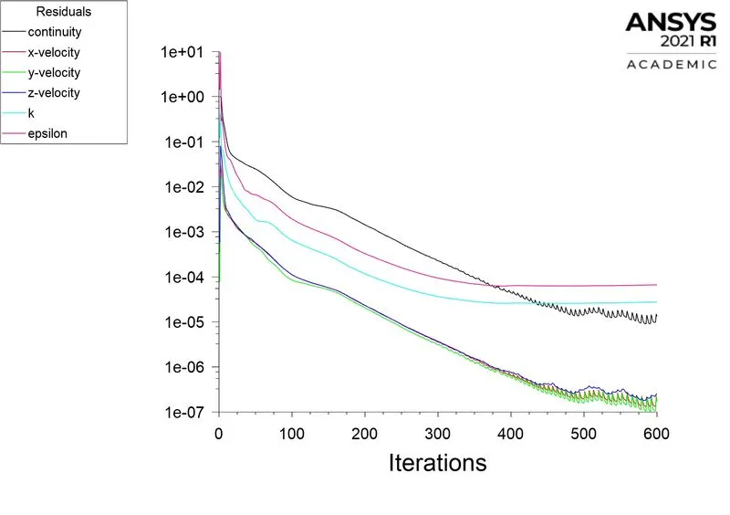
Residual Plot

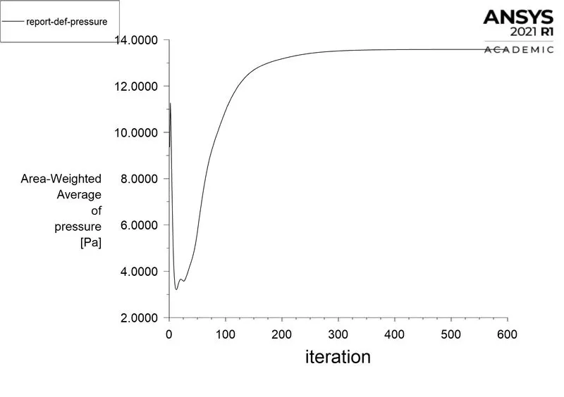
Area weighted average of Pressure

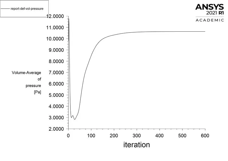
Volume average of Pressure

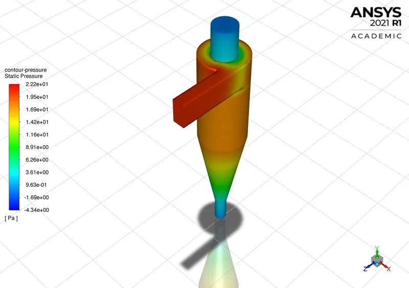
Static Pressure

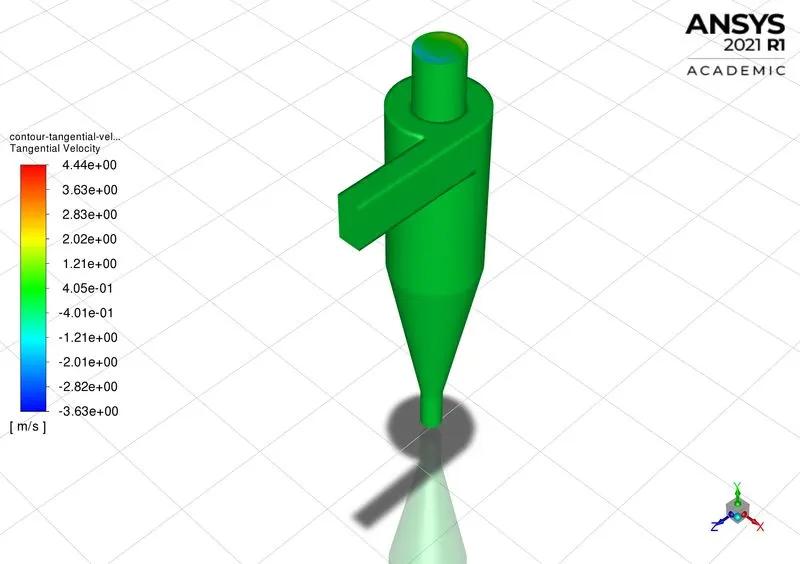
Tangential Velocity

Radial Velocity

Axial Velocity

Anthracite Particle Time

Comparison of all cases

Table-1

Mesh	Element size	Number of elements	Particle size	Inlet velocity `msec^-1`	Area weighted average of Pressure (Pa)	Volume average of Pressure (Pa)	Number of Particles tracked	Number of Particles trapped	Pressure drop (Pa)	Cyclone Efficiency `eta_(efficiency)=frac{N_(trapped)}{N_(tracked)}**100`
Refined mesh	`10mm`	`112565`	`1e-6m`	`3msec^-1`	`11.8978`	`9.3656`	`124`	`31`	`18.3194`	`25%`
	`9mm`	`141918`	`3e-6``m`		`12.6941`	`9.9649`	`142`	`125`	`19.4588`	`88.02%`
	`8mm`	`185349`	`5e-6m`		`13.5805`	`10.6312`	`172`	`165`	`20.706`	`95.93%`

Case-3

The velocity is varied from `1msec^-1` to `5msec^-1` keeping the particle size as `5e-6m`, accordingly the cyclone separator efficiency is calculated.

Refined mesh

Element size: `10mm`

Number of elements: `112565`

Particle size: `5e-6m`

Inlet velocity: `1msec^-1`

Residual Plot

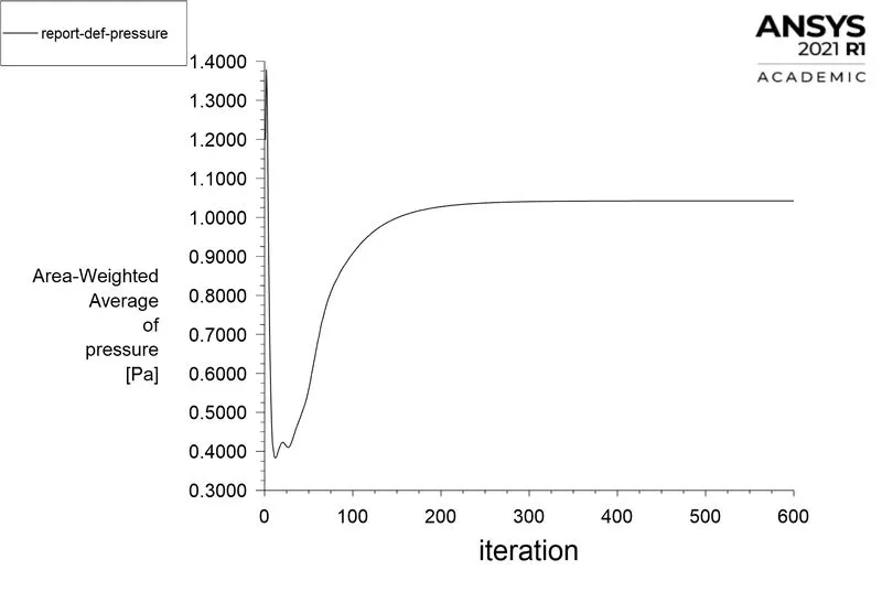
Area weighted average of Pressure

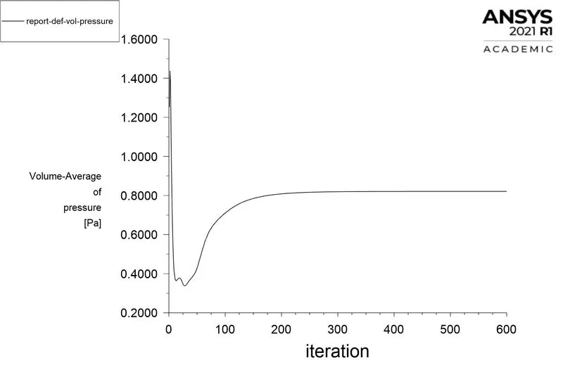
Volume average of Pressure

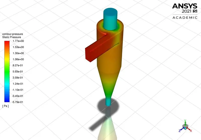
Static Pressure

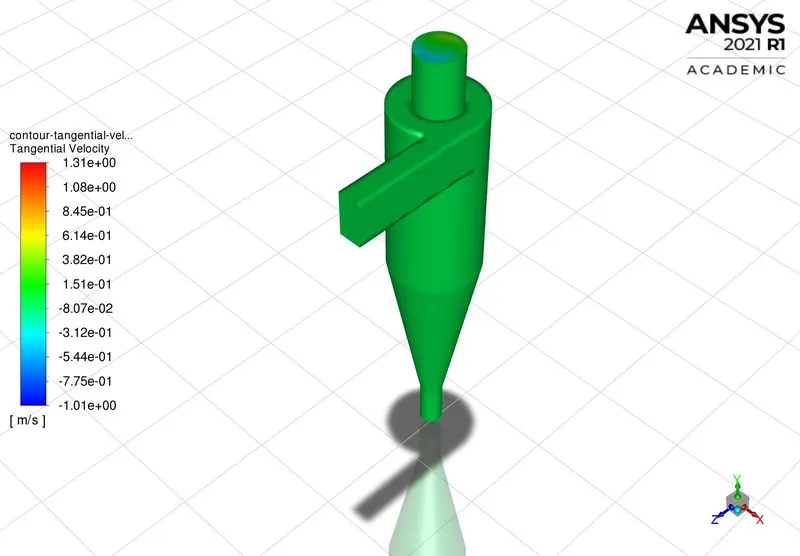
Tangential Velocity

Radial Velocity

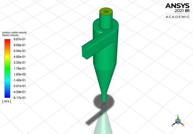
Axial Velocity

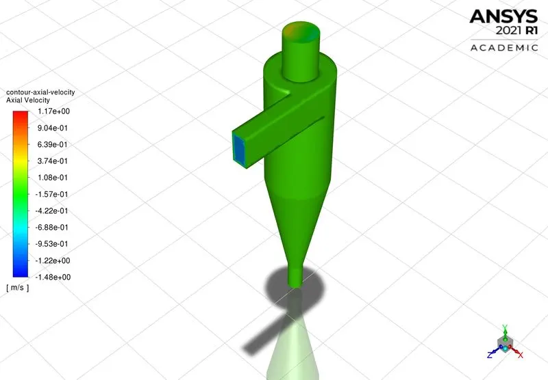
Anthracite Particle Time

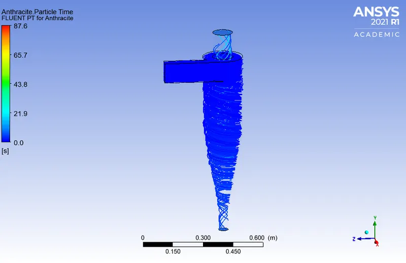
Element size: `9mm`

Number of elements: `141918`

Particle size: `5e-6m`

Inlet velocity: `3msec^-1`

Residual Plot

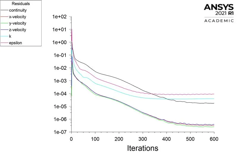
Area weighted average of Pressure

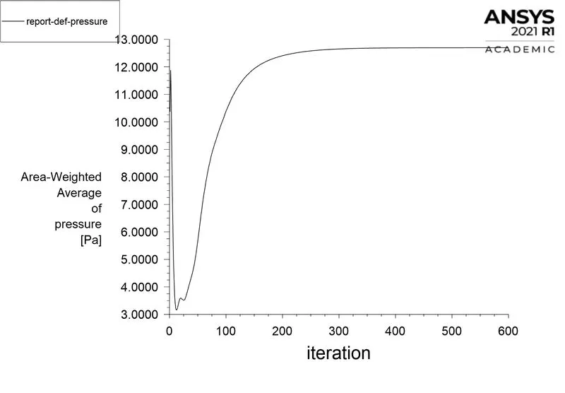
Volume average of Pressure

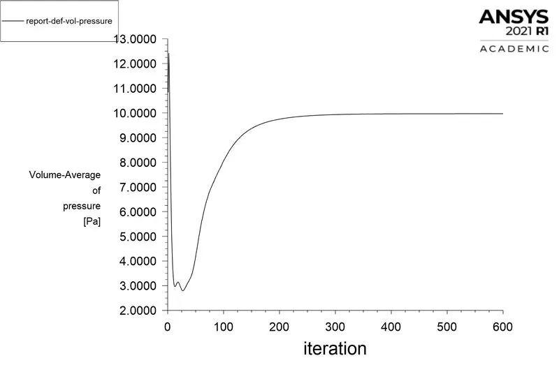
Static Pressure

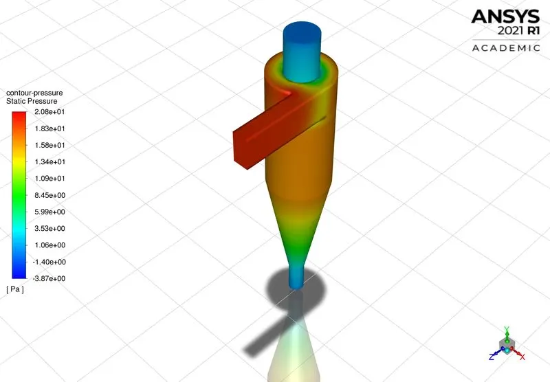
Tangential Velocity

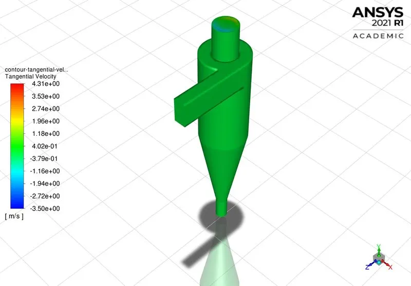
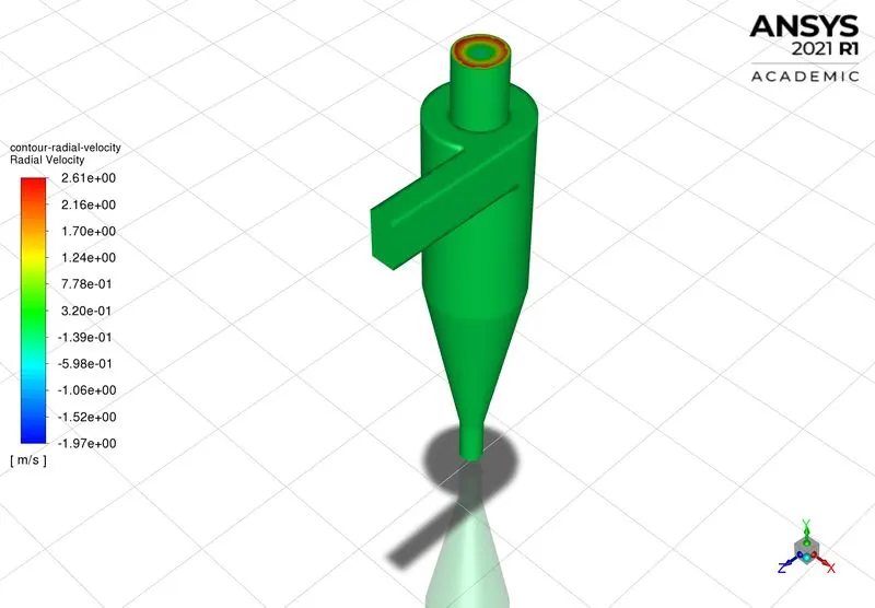
Radial Velocity

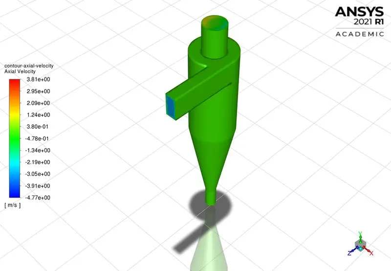
Axial Velocity

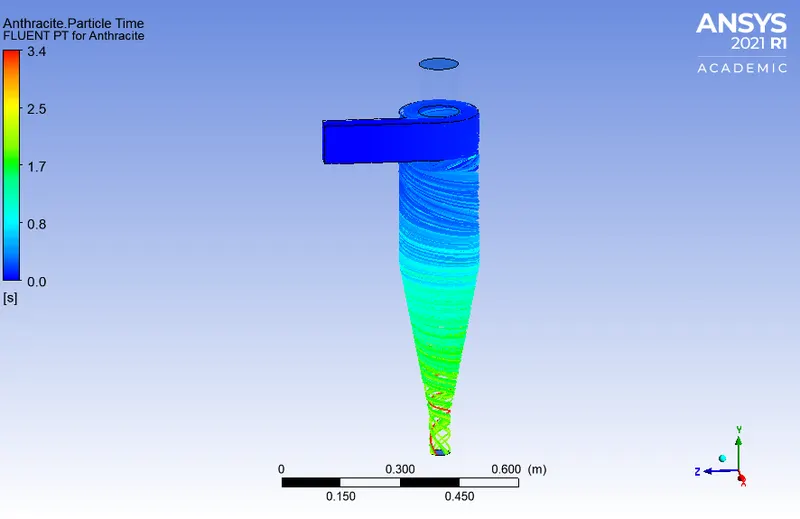
Anthracite Particle Time

Element size: `8mm`

Number of elements: `185349`

Particle size: `5e-6m`

Inlet velocity: `5msec^-1`

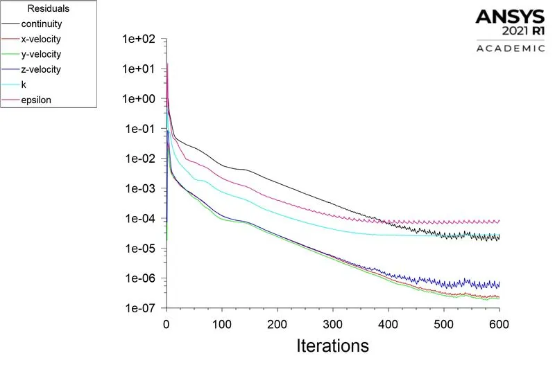
Residual Plot

Area weighted average of Pressure

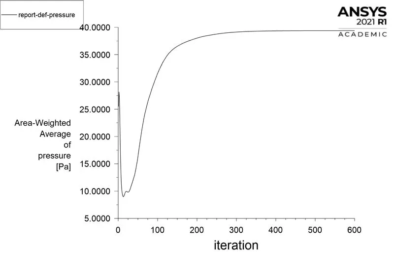
Volume average of pressure

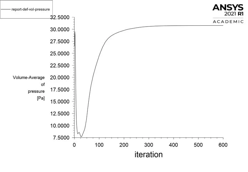
Static Pressure

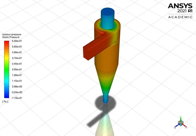
Tangential Velocity

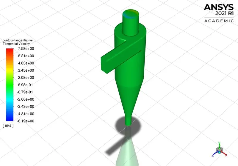
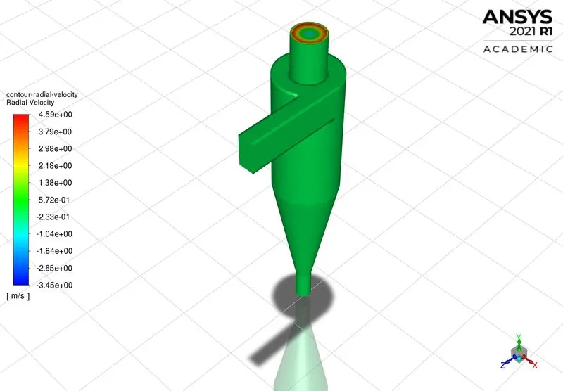
Radial Velocity

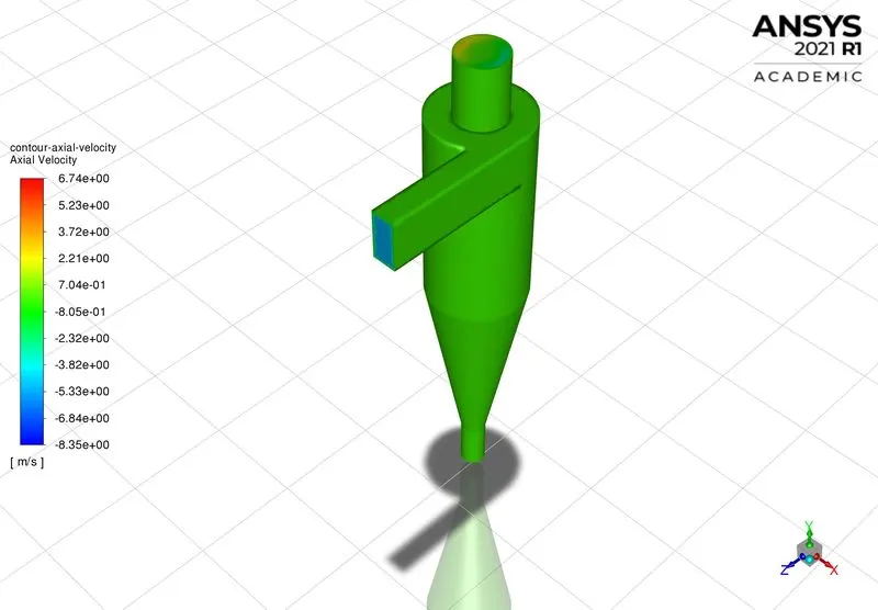
Axial Velocity

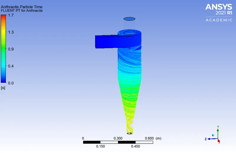
Anthracite Particle Time

Comparison of all cases

Table-2

Mesh	Element Size	Number of Elements	Particle size	Inlet Velocity `msec^-1`	Reynolds number `R_e=frac{rho**v**D}{mu}`	Area weighted average of Pressure (Pa)	Volume average of Pressure (Pa)	Pressure drop (Pa)	Number of particles tracked	Number of particles trapped	Cyclone efficiency `eta_(efficiency)=frac{N_(trapped)}{N_(tracked)}**100`
Refined mesh	`10mm`	`112565`	`5e-6m`	`1`	`13691`	`1.037094`	`0.8208813`	`1.69251`	`124`	`11`	`8.87%`
	`9mm`	`141918`		`3`	`41075`	`12.69416`	`9.964973`	`19.4588`	`142`	`142`	`100%`
	`8mm`	`185349`		`5`	`68458`	`39.38731`	`30.77455`	`59.543`	`172`	`172`	`100%`

Cyclone separator efficiency for different particle diameter sizes and same input velocity `5msec^-1`.

Table-3

Mesh	Element Size	Number of Elements	Particle size	Inlet Velocity `msec^-1`	Reynolds number `R_e=frac{rho**v**D}{mu}`	Area weighted average of Pressure (Pa)	Volume average of Pressure (Pa)	Pressure drop (Pa)	Number of particles tracked	Number of particles trapped	Cyclone efficiency `eta_(efficiency)=frac{N_(trapped)}{N_(tracked)}**100`
Refined mesh	`8mm`	`185349`	`1e-6m`	`5`	`68458`	`39.38731`	`30.77455`	`59.543`	`172`	`49`	`28.48%`
			`3e-6m`			`39.38731`	`30.77455`		`172`	`169`	`98.25``%`
			`5e-6m`			`39.38731`	`30.77455`		`172`	`172`	`100%`

Conclusion

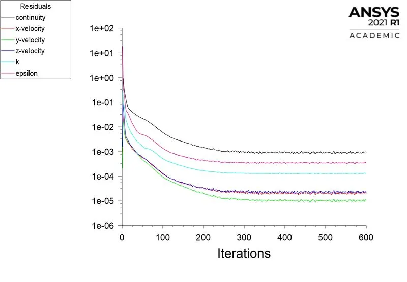
• The steady-state simulation was performed with COUPLED pressure-velocity coupling schemes and the monitor plot showed that the graph is stable and in each case, for the refined mesh it takes 300 iterations to converge and after that solution acquires a steady-state.
• The `k-epsilon` `RNG` swirl dominated flow and near-wall treatment as standard wall function was selected for improving the accuracy of the solution.
• The velocity contour (axial, radial, tangential) and static pressure contour, anthracite particle time have been plotted for each case.
• The number of particles tracked, trapped, cyclone separator efficiency, and the pressure drop were tabulated for each case.
• The cyclone separator efficiency was evaluated by `eta_(efficiency)=frac{N_(trapped)}{N_(tracked)}**100`.
• The Reynolds number increases with an increase in input velocity given by the formula `R_e=frac{rho**v**D}{mu}` where D is the diameter of the cyclone separator which is `0.2m`
• The pressure drop in the cyclone separator was visualized as entry pressure loss, accompanied by the friction loss due to the swirling motion of the particle-laden air, the change in direction of airflow from outlet_top to outlet_bottom. In general cases the pressure drop is calculated in CFD post by the expression areaAvgPressure(@inlet)-areaAvgPressure(@outlet_bottom), the same has been tabulated for each case.
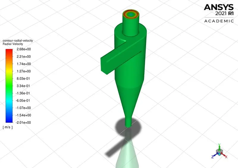
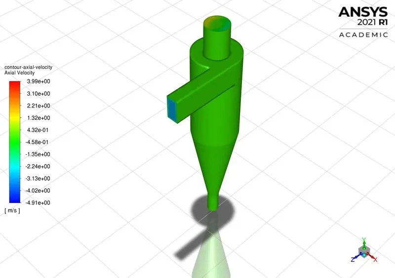
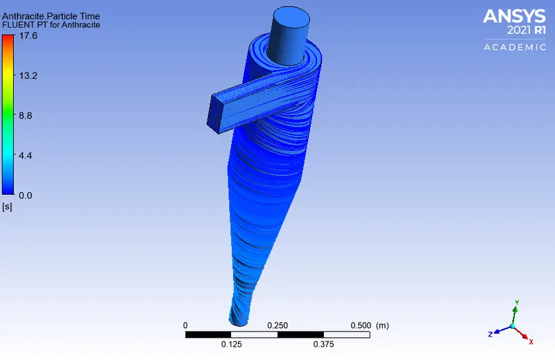
• It can be concluded from Table-1 that by changing the particle size from `1e-6m` to `5e-6m` and keeping the velocity as `3msec^-1`, the inertia of the particle increases and which further decreases the anthracite particle time. As the inertia of the particle increases, more particles get trapped at the bottom which results in a steady rise in cyclone separator efficiency which indicates the range under which the cyclone separator model will work appropriately. Since the inlet velocity is constant in each case the velocity contour plots ( axial, radial, tangential) and static pressure contour plots do not show significant differences as tabulated under heading Table-1.
• It can be concluded from Table-2 that by varying the inlet velocity (`1msec^-1`, `3msec^-1`, `5msec^-1`) keeping the particle size as `5e-6m` the anthracite particle time is maximum for `1msec^-1` and it is less for `5msec^-1` the reason being that the anthracite particle time is inversely related to the velocity as such when the velocity is `5msec^-1` the time taken by the particle-laden air to transverse the distance from inlet to outlet is less. Moreover, as the velocity increases from `1msec^-1`to `3msec^-1` there is a considerable increase in cyclone separator efficiency from `8.87%` to `100%` can be attributed to the fact that as the velocity increases the exchange of momentum increases from the dispersed phase to the fluid phase leading to the increase in efficiency of the cyclone separator. Moreover, for the element size, 8mm the efficiency of the cyclone separator is `100%` because the velocity of the particle increases to `5msec^-1`which imparts momentum to the fluid thus resulting in heavier particles being collected at the bottom.
• The air containing anthracite is fed into the inlet section of the cyclone separator, the air experiences the swirling motion and by the principle of vortex separation, the anthracite particle is collected at the bottom, in the process of doing so some of the particles hit the wall of the cyclone separator which makes the particle velocity to be `0msec^-1` justifying the no-slip condition of the wall. The tangential velocity decreases with an increase in radius of the inner vortex and increases with a decrease in radius of the outer vortex.
• The number of particles tracked depends on the refined mesh.
• The particle size and the input velocity greatly impacted the efficiency of the cyclone separator thus providing the basis for the design and analysis for the same.

SOURCE: https://www.researchgate.net/publication/232747389_A_CFD_Study_on_the_Prediction_of_Cyclone_Collection_Efficiency