UNDERSTANDING THE STABILITY ANALYSIS IN LINEAR SYSTEM THROUGH ITERATIVE METHODS

Aim: To understand the stability of the linear system using iterative techniques

Abstract

In the above case, eigenvalues of [3 x 3] matrix are calculated by using iterative methods. The inbuilt command will not be used in this case.

Governing equation:

Let us consider a general [] 3 X 3 matrix which is of the form

• Coefficient matrix,`A=[[a11,a12,a13],[a21,a22,a23],[a31,a32,a33]]`

The coefficient matrix is decomposed into diagonal matrix "D", lower triangular matrix "L", upper triangular matrix "U".

Therefore,

`D=[[a11,0,0],[0,a22,0],[0,0,a33]]`

`L=[[0,0,0],[a21,0,0],[a31,a32,0]]`

`U=[[0,a12,a13],[0,0,a23],[0,0,0]]`

So, coefficient matrix, `A= L+U+D`

The general system of linear equation is `AX=B`

Iterative methods

• Jacobi method

It uses the old value of the iteration and update the new value after iteration after it has transferred the entire array. So when `AX=B`is solved for the Jacobi method the result yields

`[[a11,a12,a13],[a21,a22,a23],[a31,a32,a33]]**[[x1],[x2],[x3]]=[[b1],[b2],[b3]]`

`a11**x1=b1-a12**x2-a13**x3`(Initially x1=0;x2=0;x3=0)

Rewriting the above equation as

`a11**x1^(n ew)=b1-a12**x2^(old)-a13**x3^(old)`

Similarly the other equation is written as

`a22**x2^(n ew)=b2-a21**x1^(old)-a23**x3^(old)`

`a33**x3^(n ew)=b3-a31**x1^(old)-a32**x2^(old)`

Writing in matrix form

`D**X^(n ew)=B-(U+L)**X^(old)`

Multiplying by `D^-1`

`D^-1D**X^(n ew)=D^-1B-D^-1(U+L)**X^(old)`

The Jacobi method is rewritten in the general iterative equation of the form

`X^(n ew)=T**X^(old)+C`

`X^(n ew)` = Current iteration value

`X^(old)` = Previous iteration value

`T` = Iteration matrix

`C` = Constant matrix

Thus the final equation for the Jacobi method is

`X^(n ew)=D^-1B-D^-1(U+L)**X^(old)`

Comparing final equation for Jacobi method to general iterative equation

`T=-D^-1(U+L)`

`C=D^-1B`

• Gauss-Seidel method

Gauss-Seidel method readily uses the updated value after it has been computed and thus it is much faster.

`[[a11,a12,a13],[a21,a22,a23],[a31,a32,a33]]**[[x1],[x2],[x3]]=[[b1],[b2],[b3]]`

`a11**x1^(n ew)=b1-a12**x2^(old)-a13**x3^(old)`

`a22**x2^(n ew)=b2-a21**x1^(n ew)-a23**x3^(old)`

`a22**x2^(n ew)+a21**x1^(n ew)=b2-a23**x3^(old)`

`a33**x3^(n ew)+a31**x1^(n ew)+a32**x2^(n ew)=b3`

Writing in matrix form

`(L+D)**X^(n ew)=B-U**X^(old)`

Multiplying by `(L+D)^(-1)`

`X^(n ew)=B**(L+D)^(-1)-U**(L+D)^(-1)**X^(old)`

Comparing the final equation for the Gauss-Seidel method to the general iterative equation

`T=-U**(L+D)^(-1)`

`C=B**(L+D)^(-1)`

• Successive over-relaxation method

It is faster than the above two iterative methods because it uses a relaxation factor called `omega`

The general iterative equation for the successive over-relaxation method is

`X^(n ew)=(L+frac{1}{omega}**D)^(-1)[(frac{1}{omega}**D-D-U)**X^(old)+B]`

`T=(L+frac{1}{omega}**D)^(-1)(frac{1}{omega}**D-D-U)`

Please note that the primary concern is the iteration matrix in all the three iterative method

The characteristics equation for finding the eigenvalues of a 3 X 3 matrix is

`lambda^3-(traceA)**lambda^2+`(sum of minor of all the diagonal elements)`**lambda-det(T)=0`

Eigenvalue, `lambda``=max(ab s(ro o ts(poly(T))))`

`T` can be Tjac, Tgs, Tsor

Spectral radius can be calculated by using the formula as under

`rho=max(abs(lambda1),abs(lambda2),abs(lambda3),abs(lambda4)...)`

Calculating eigenvalue and spectral radius for diagonal modification DM=0.5

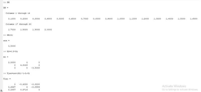
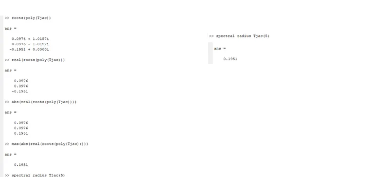
Diagonally dominant matrix

The matrix is said to be diagonally dominant if the magnitude of the diagonal entry in a row is larger than or equal to the sum of the magnitudes of all the other (non-diagonal) entries in that row.

Let us consider the square matrix A

`A=[[a11,a12,a13],[a21,a22,a23],[a31,a32,a33]]`

`abs[a11]ge(a12+a13)`

`abs[a22]ge(a21+a23)`

`abs[a33]ge(a31+a32)`

Diagonal dominance plays an important role in the "CFD" solution. Thus when a matrix is diagonally dominant the solution will converge faster. The diagonal dominance and the spectral radius will tell us whether the solution will converge or not thus an important criterion determining the stability analysis of the linear system.

Matlab coding procedures

• Gathering all the input parameters viz A, L, D, U, B as given in the problem.
• Assigning diagonal modification to the diagonal matrix
• Creating a for loop for calculating eigenvalues and spectral radius.
• Calculating iteration matrix for all the three iterative methods.
• Calculating eigenvalues by using a command called poly
• Calculating the maximum of the real values of the eigenvalues to calculate the spectral radius of the given iteration matrix
• Calling user-defined function to calculate the iteration.
• For loop ends.
• The graph is plotted between (diagonal modification and spectral radius), (spectral radius and number of iterations).

Matlab code

• Creating a Matlab code to understand the stability analysis in a linear system.

clear
close all
clc

% coefficient matrix
A=[5 1 2;-3 9 4;1 2 -7];
% lower triangular matrix
L=[0 0 0;-3 0 0;1 2 0];
% upper triangular matrix
U=[0 1 2;0 0 4;0 0 0];
% diagonal matrix
D1=[5 0 0;0 9 0;0 0 -7];

% right hand side
B=[10;-14;33];
% identity matrix
I=[1 0 0; 0 1 0;0 0 1];

% omega
omega=1.25;


% diagonal modification
DM=(1:1:10);
for i=1:length(DM)
    D=D1*DM(i);
    % iteration matrix for jacobi
   
    Tjac=inv(D)*(-L-U);
    eigen_value_Tjac=roots(poly(Tjac));
    spectral_radius_Tjac(i)=max(abs(real(eigen_value_Tjac)));
    % calling jacobian function
    [jac_iter(i),X]=jacobi(L,D,U,B);
   
    % iteration matrix for gauss-seidel method

    Tgs=-U*inv(L+D);
    eigen_value_Tgs=roots(poly(Tgs));
    spectral_radius_Tgs(i)=max(abs(real(eigen_value_Tgs)));
    % calling gauss-seidel function
    [GS_iter(i),X]=GS(L,D,U,B);
  
    % iteration matrix for successive over relaxation method
    
    Tsor=inv(D+(omega*L))*(((1-omega)*D)-(U*omega));
    eigen_value_Tsor=roots(poly(Tsor));
    spectral_radius_Tsor(i)=max(abs(real(eigen_value_Tsor)));
    % calling SOR method
    
    [SOR_iter(i),X]=SOR(L,D,U,B);
    
end
    % plotting
    figure(1)
    subplot(2,1,1)
    plot(DM,spectral_radius_Tjac)
    grid on
    xlabel('diagonal modification')
    ylabel('spectral radius Tjac')
    title('Jacobi Method')
    
    
   
    subplot(2,1,2)
    plot(spectral_radius_Tjac,jac_iter)
    grid on 
    xlabel('spectral radius')
    ylabel('Number of jacobi iteration')
    
    figure(2)
    subplot(2,1,1)
    plot(DM,spectral_radius_Tgs)
    grid on
    xlabel('diagonal modification')
    ylabel('spectral radius Tgs')
    title('GS Method')
    
    subplot(2,1,2)
    plot(spectral_radius_Tgs,GS_iter)
    grid on 
    xlabel('spectral radius')
    ylabel('Number of GS iteration')
    figure(3)
    subplot(2,1,1)
    plot(DM,spectral_radius_Tsor)
    grid on
    xlabel('diagonal modification')
    ylabel('spectral radius Tsor')
    title('SOR Method')
    
    subplot(2,1,2)
    plot(spectral_radius_Tsor,SOR_iter)
    grid on 
    xlabel('spectral radius')
    ylabel('Number of SOR iteration')

• Calling user-defined functions

function [jac_iter,X]=jacobi(L,D,U,B)
error=9e9;
tol=1e-4;
jac_iter=1;
Xold=[0;0;0];

    % jacobi iteration
    while(error>tol)
    X=inv(D)*B+(inv(D)*(-L-U)*Xold);
    
    error=max(abs(Xold-X));
    Xold=X;
    jac_iter=jac_iter+1;
    end
    
end

function [GS_iter,X]=GS(L,D,U,B)
error=9e9;
tol=1e-4;
GS_iter=1;
Xold=[0;0;0];

    % GS
    while(error>tol)
    X=inv(L+D)*B+(inv(L+D)*(-U)*Xold);
    
    error=max(abs(Xold-X));
    Xold=X;
    GS_iter=GS_iter+1;
    end
    
end

function [SOR_iter,X]=SOR(L,D,U,B,omega)
error=9e9;
tol=1e-4;
SOR_iter=1;
Xold=[0;0;0];
I=[1 0 0; 0 1 0;0 0 1];



    % SOR
    while(error>tol)
    X=((1-omega)*Xold+(omega*((inv(D+L)*B)+inv(D+L)*(-U)*Xold)));
    
    error=max(abs(Xold-X));
    Xold=X;
    SOR_iter=SOR_iter+1;
    end
    
end

• Output graph

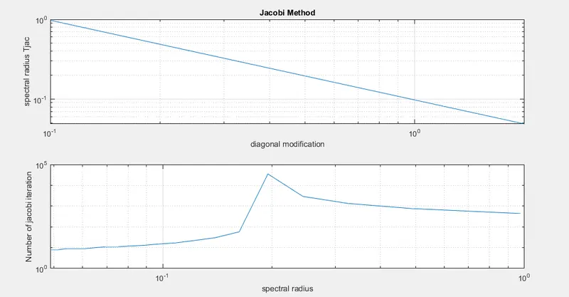
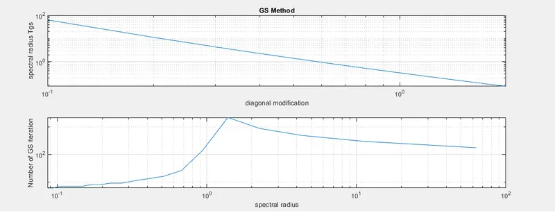
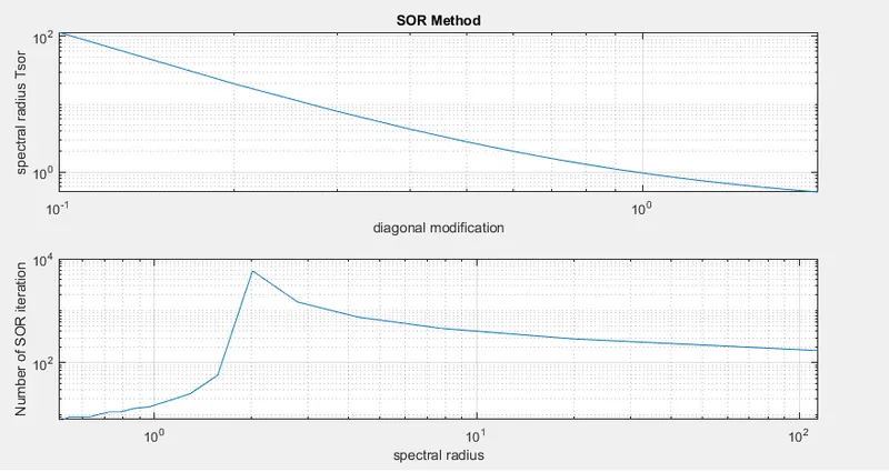
Conclusion

It can be concluded from the graphs and the table that

• The diagonal modification and spectral radius are inversely related to each other. As diagonal modification increases the value for spectral radius tends to decrease. The lower diagonal modification value will yield a larger value of the spectral radius, as such there will be large iteration values for which Matlab produces the result as NaN. The fall of the spectral radius is rapid in the successive over-relaxation method.
• For the solution to converge the spectral radius has to be less than 1. If the spectral radius is greater than one the solution will not converge.
• In the second subplot, in the region where the spectral radius is less than 1 the number of iteration required for convergence of solution also decreases.
• The region where the spectral radius is greater than one is of less significance.