Week 8 - Simulating Cyclone separator with Discrete Phase Modelling
Aim:- To perform analysis on cyclone separator and calculate the separation efficiency and pressure drop.
Objective:-
- To write a few words about any four empirical models used to calculate the cyclone separator efficiency.
- To perform an analysis on a given cyclone separator model by varying the particle diameter from 1 μm to 5 μm and calculate the separation efficiency in each case. Discuss the results. [Use both the velocity's as 3m/sec.]
- To perform an analysis on a given cyclone separator model by varying the particle velocity from 1 m/sec to 5 m/sec and calculate the separation efficiency and pressure drop in each case. Discuss the results. [Use particle diameter size as 5 μm for all cases & keep flow velocity same as particle velocity]
THEORY:
CYCLONE SEPERATORS:
Cyclone separators provide a method of removing particulate matter from air or other gas streams at low cost and low maintenance. Cyclones are somewhat more complicated in design than simple gravity settling systems, and their removal efficiency is much better than that of settling chamber. Cyclones are basically centrifugal separators, consists of an upper cylindrical part referred to as the barrel and a lower conical part referred to as cone. They simply transform the inertia force of gas particle flows to a centrifugal force by means of a vortex generated in the cyclone body. The particle laden air stream enters tangentially at the top of the barrel and travels downward into the cone forming an outer vortex. The increasing air velocity in the outer vortex results in a centrifugal force on the particles separating them from the air stream. When the air reaches the bottom of the cone, it begins to flow radially inwards and out the top as clean air/gas while the particulates fall into the dust collection chamber attached to the bottom of the cyclone.
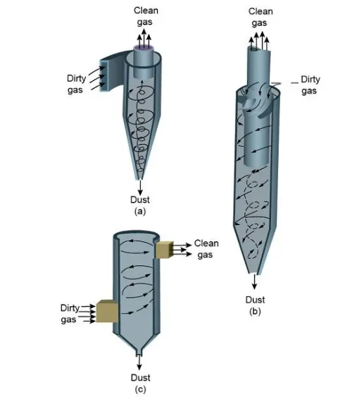
The collection efficiency of cyclones varies as a function of density, particle size and cyclone design. Cyclone efficiency will generally increase with increases in particle size and/or density; inlet duct velocity; cyclone body length; number of gas revolutions in the cyclone; ratio of cyclone body diameter to gas exit diameter; inlet dust loading; smoothness of the cyclone inner wall.Similarly, cyclone efficiency will decrease with increases in the parameters such as gas viscosity; cyclone body diameter; gas exit diameter; gas inlet duct area; gas density; leakage of air into the dust outlet.
The efficiency of a cyclone collector is related to the pressure drop across the collector. This is an indirect measure of the energy required to move the gas through the system. The pressure drop is a function of the inlet velocity and cyclone diameter. Form the above discussion it is clear that small cyclones are more efficient than large cyclones. Small cyclones, however, have a higher pressure drop and are limited with respect to volumetric flow rates.
CYCLONE SEPERATOR EMPERICAL MODELS
-
Iozia and Leith ModelIozia and Leith [4] logistic model is a modified version of Barth Model, which is developed based on force balance.The model assumes that a particle carried by the vortex endures the influence of two forces: a centrifugal force, Z and a flow resistance, W . The collection efficiency η of particle diameter d can be calculated from
ηi=11 + (dpc/dpi)ββ is an expression for slope parameter -
Koch and Licht ModelKoch and Licht collection theory recognized the inherently turbulent nature of cyclones and the distribution of gas residence times within the cyclone. Koch and Licht described particle motion in the entry and collection regions with the additional following assumptions:• The tangential velocity of a particle is equal to the tangential velocity of the gas flow, i.e. there is no slip in the tangential direction between the particle and the gas.•The tangential velocity is related to the radius of cyclone by: u Rn= constant.A force balance and an equation on the particles collection yieldsthe grade efficiencyηi= 1 − exp{−2[GτiQ/D3*(n + 1)]^(0.5/(n+1))}
G =8Kc/[(Ka^2)*(Kb^2)] -
Lapple ModelLapple model was developed based on force balance without considering the flow resistance. Lapple assumed that a particle entering the cyclone is evenly distributed across the inlet opening. The particle that travels from inlet half width to the wall in the cyclone is collected with 50% efficiencyηi=1/[1 + (dpc/(dpi^2))]
-
Li and Wang Model
The Li and Wang [3] model includes particle bounce or re-entrainment and turbulent diffusion at the cyclone wall. A two-dimensional analytical expression of particle distribution in the cyclone is obtained. Li and Wang model was developed based on the following assumptions:
• The radial particle velocity and the radial concentration profile are not constant for uncollected particles within the cyclone.
• Boundary conditions with the consideration of turbulent diffusion coefficient and particle bounce re-entrainment on the cyclone wall.
• The tangential velocity is related to the radius of cyclone by: u Rn= constant.
The resultant expression of the collection efficiency for particle of any size is given as
ηi= 1 − exp{−λθ1}
where
θ1= 2π (S + L)/a
DISCRETE PHASE MODELLING :
A discrete phase model (DPM) is used when the aim is to investigate the behavior of the particles from a Lagrangian view and a discrete perspective. In fact, the difference between the Lagrangian and the Eulerian view is that fluid behavior in Lagrangian view is examined on the basis of a particle tracking of a particle of fluid flow; Whereas fluid behavior is considered in Eulerian view based on the assumption of a finite volume element in the fluid flow path.
If the behavior of discrete particles in the presence of a continuous flow field is affected by continuous flow, the interaction with the continuous phase must be activated. Also, if the particle tracking is relatively unsteady over time, the unsteady particle tracking option must be activated. The discrete phase can be applied in various physical forms, the type of which depends on the problem model. continuous- consists of fluid flowing the fluid volume; discrete- smaller particles association with the fluid
Also, the injection process for the mixed flow is defined in the input section of the model. In this way, in the input section of the model, the desired material enters the interior space of the model with the same discrete state or particle by particle. This particle injection as a discrete state can occur in different states. For example, the combusting mode is used when the material is injected into the model’s interior to perform the combustion process.
Boundary Conditions:-
Inlet and wall:- Reflect
Outlet(Top):- Escape
Outlet(Bottom/dustbin) - Trap
CASE 1:Inject velocity 3m/s and particle size is 5Micrometer
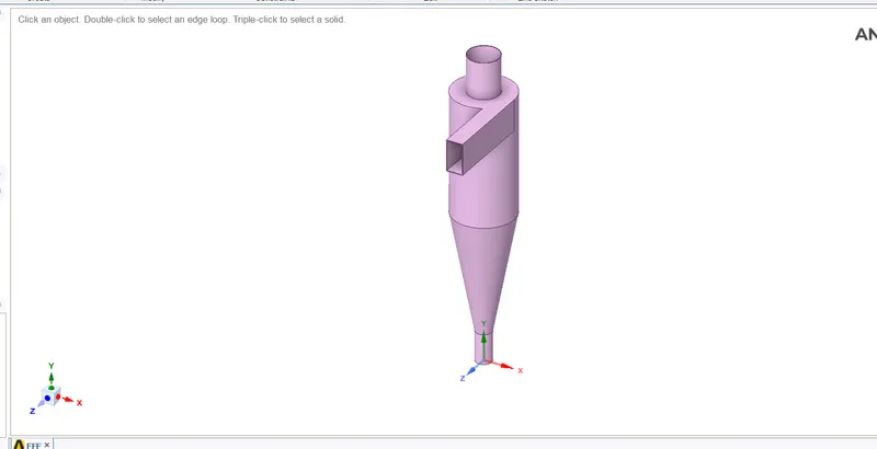
Opened the model in spaceclaim
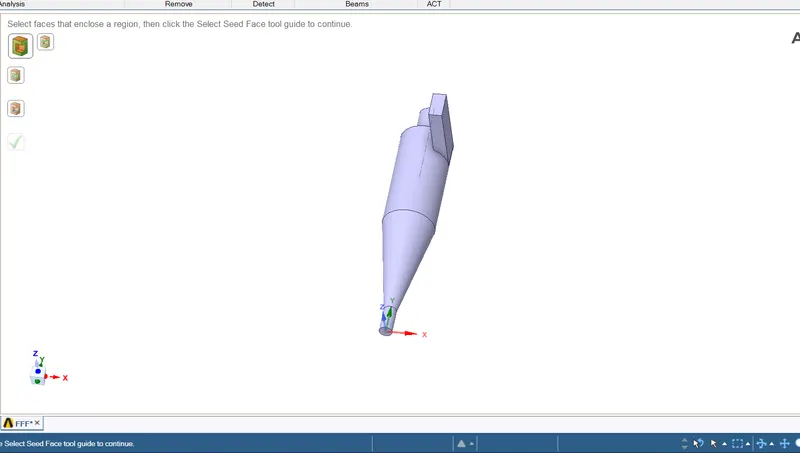
Volume extracted
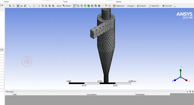
Meshing done by using default mesh
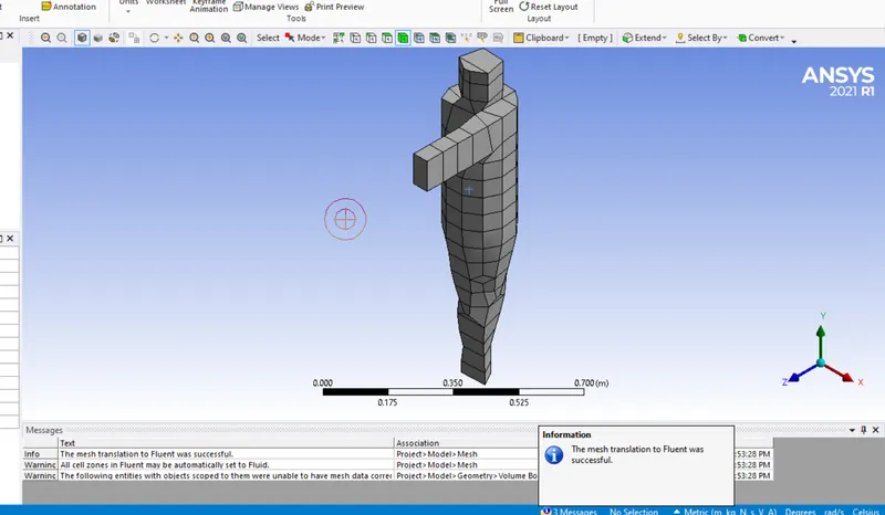
Cartesian meshing done
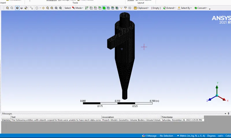
Meshing done with 5mm mesh
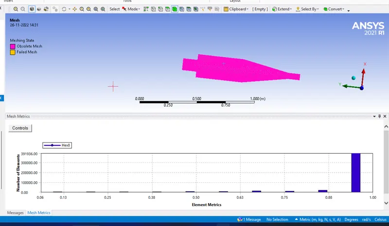
Checking mesh quality
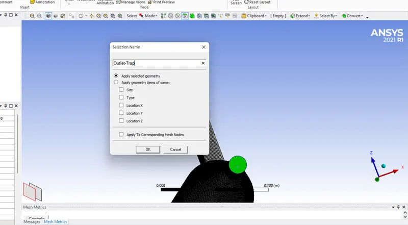
Giving naming
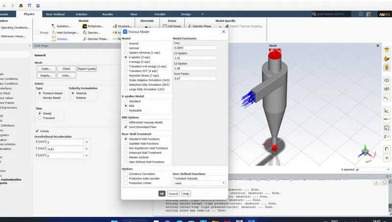
Giving turbulence model
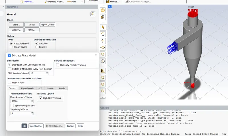
Giving DPM Model
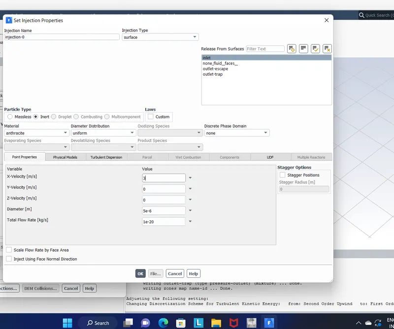
Giving particle size and velocity
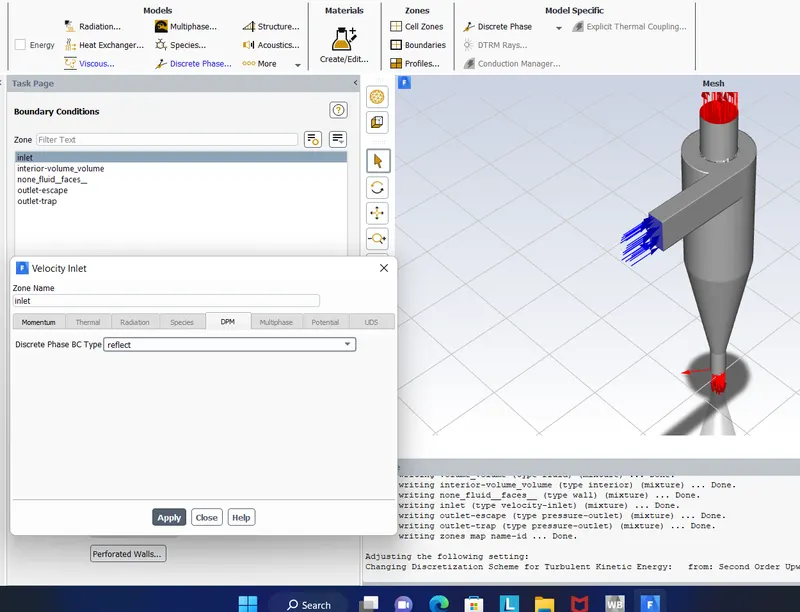
Giving inlet boundary conditions
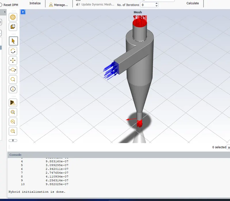
Hybrid Initialization done
RESULTS AND DISCUSSIONS:
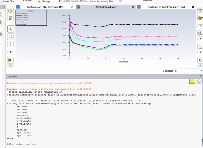
Showing Residuals
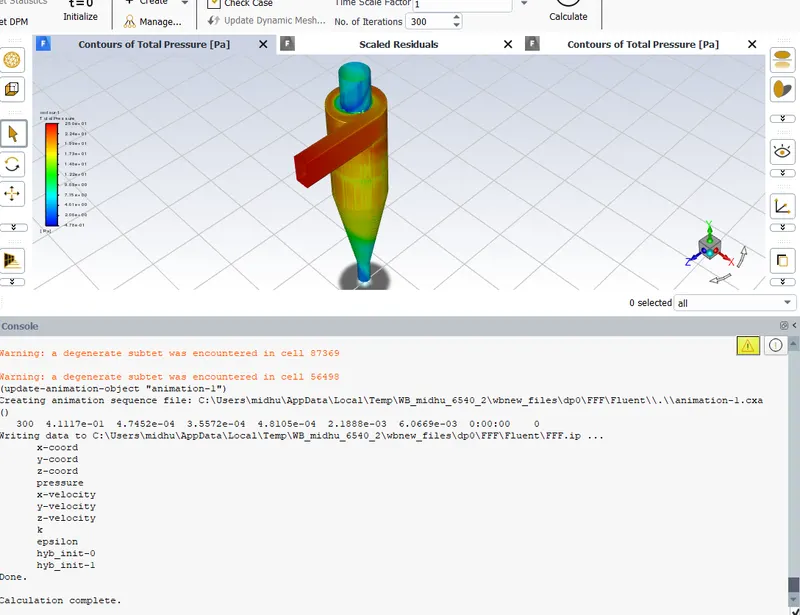
Showing contour of total pressure
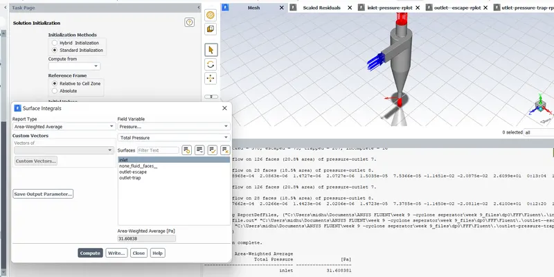
Area weighted average of total pressure at inlet is31.608 Pa
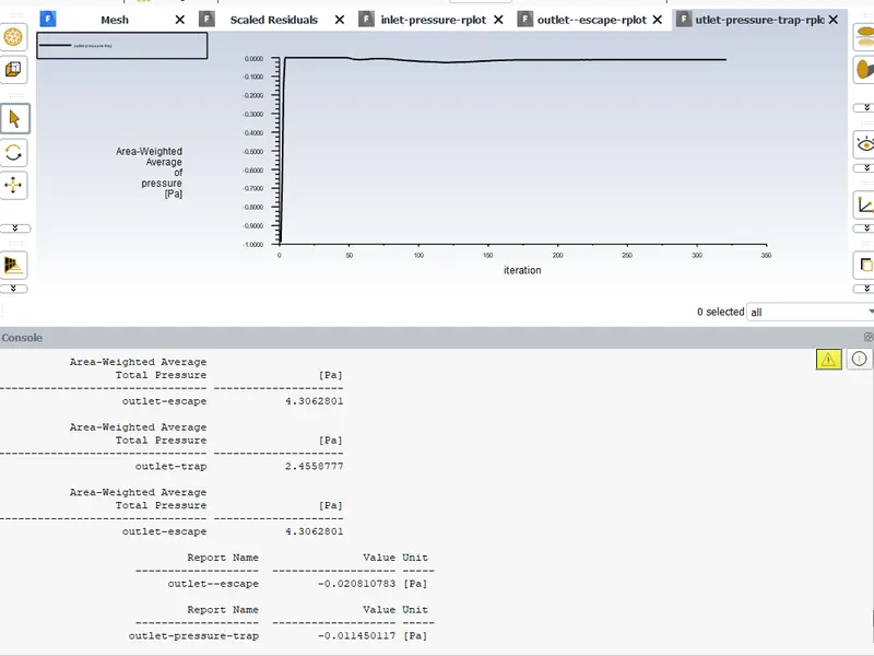
Area weighted average of pressure at outlet is 0.02 Pa
Therefore here pressure drop is 31.608-0.02= 31.588Pa
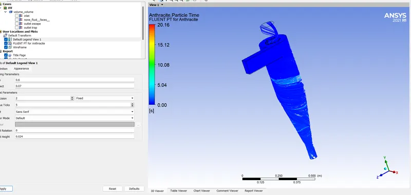
Showing contour of particle time
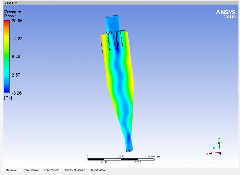
Showing contour of pressure.
It is clear that pressure is minimum at the centre of cyclone seperaator and maximum near the walls.
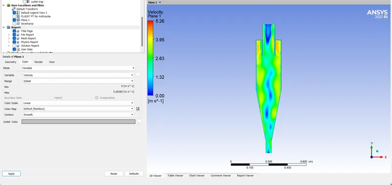
Showing contour of pressure.
It is clear thatvelocity also minimum at the centre of cyclone seperaator and maximum near the walls beacuse particles are rotating near the walls due to centrifugal force and this velocity is pulling the particles towars centre of cyclone sepertor and finally particles will settle at the bottom.
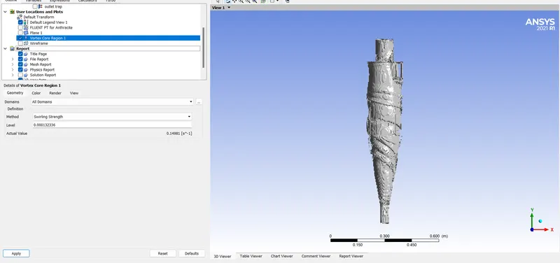
This vortex core region shows the swirling phenomena inside the cyclone seperator
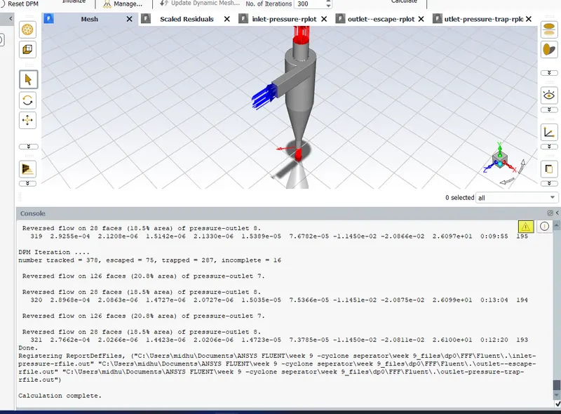
Details showing no of particles trapped, escaped and incomplete.
Here, no of particles tracked = 378
no of particles trapped = 287
no of particles escaped = 75
no of particles incomplete = 16
Seperator Tracking Efficiency = (no of particles trapped/no of particles tracked ) X 100= (287/378)X 100 = 75.92%
NOTE: Video for total pressure is uploaded below
CASE 2: Injecting velocity =3m/s and Particle size 3 Micrometer
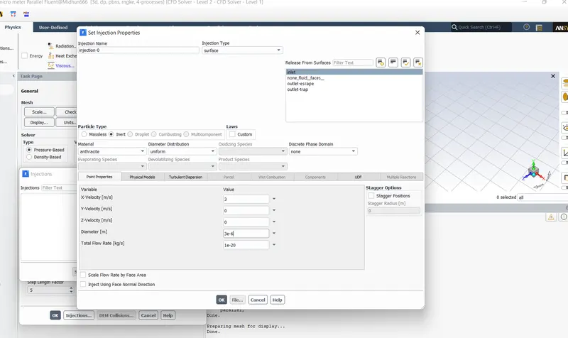
Giving injecting velocity and particle size
RESULTS AND DISCUSSIONS:
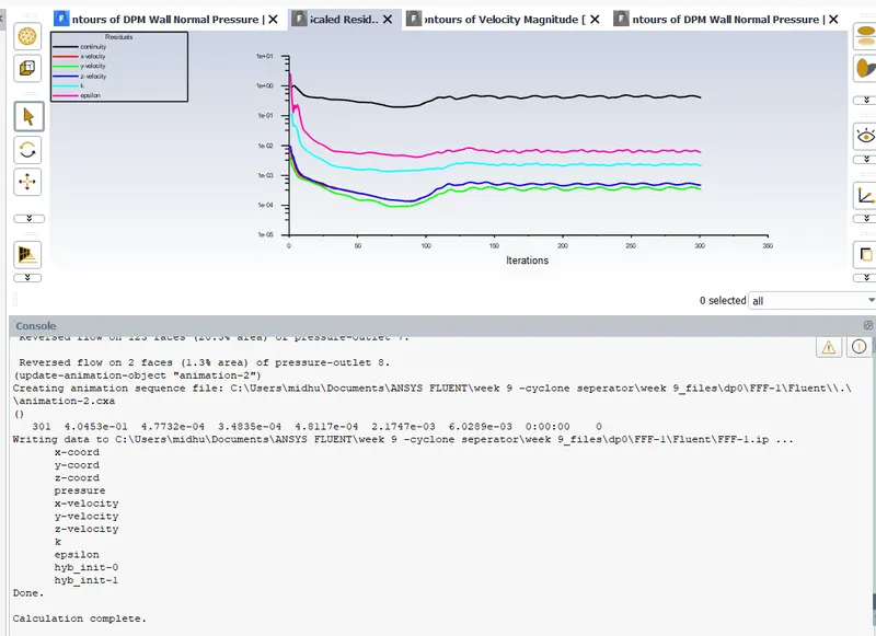
Showing residuals
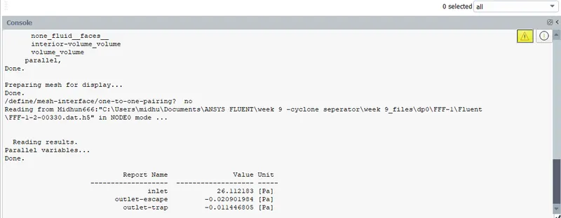
Showing total pressure at inlet as 26.112 Pa
Total pressure at outlet escape as 0.02Pa
So, the total pressure drop = 26.112-0.02 = 26.092 Pa
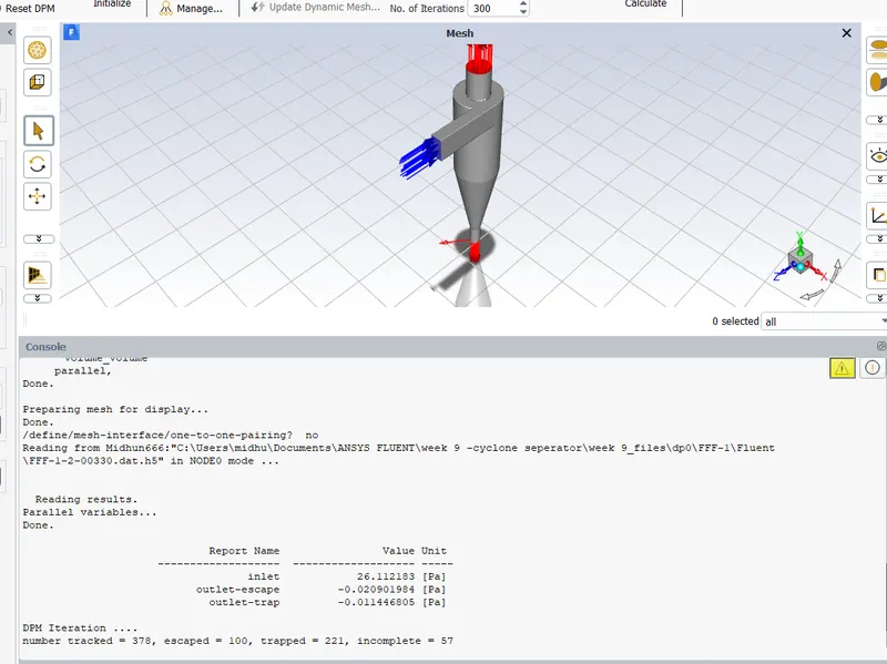
No of particles tracked = 378
No of particles trapped = 221
No of particles escaped = 100
No of particles incomplete = 57
So, tracking efficiency = (221/378)X 100 = 58.46%
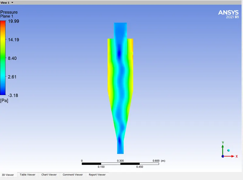
Showing pressure contour
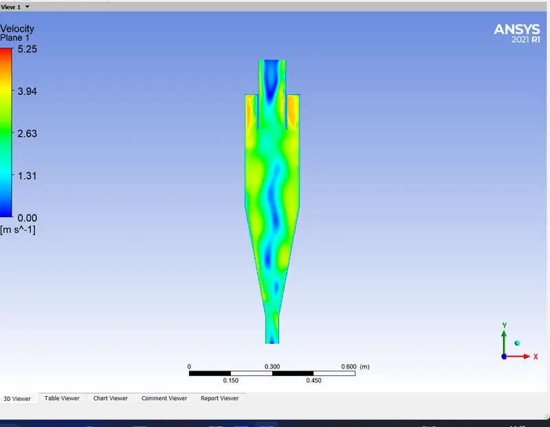
Showing velocity contour
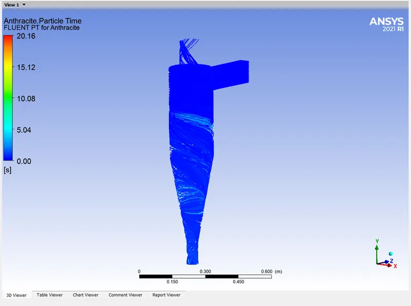
Showing particle time
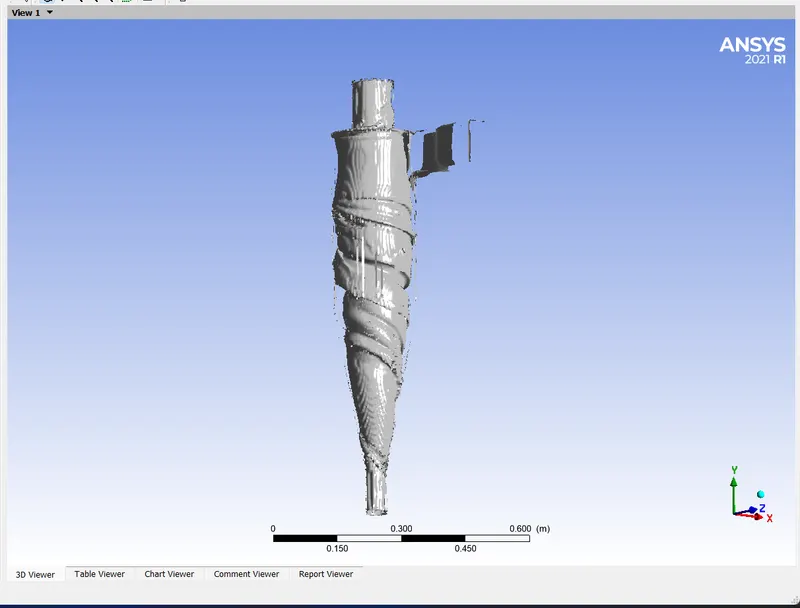
Showing vortex core region which shows swirling phenomena inside the seperator
CASE 3: Inject velocity 3m/s and particle size 1Micrometer
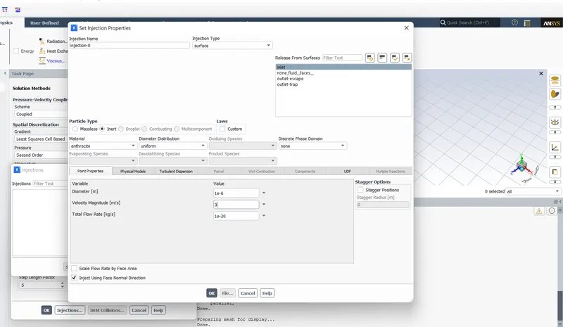
Giving inject velocity and particle size
RESULTS AND DISCUSSIONS:
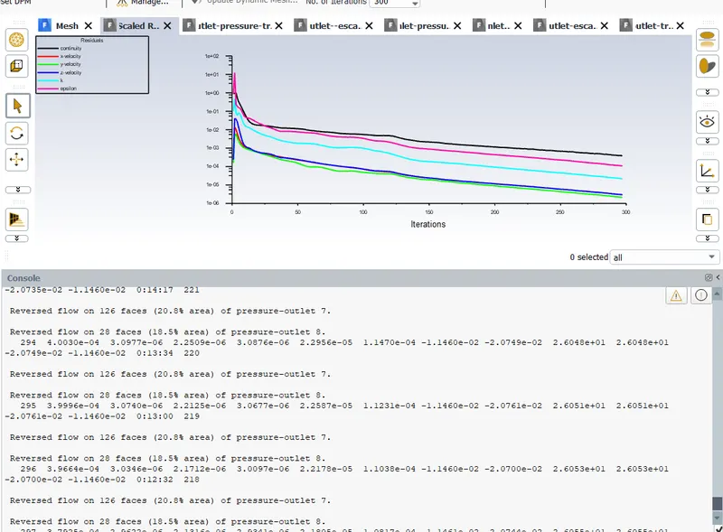
Showing residuals
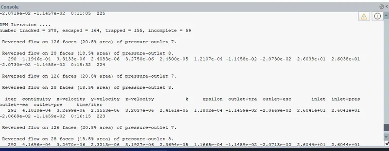
No of particles tracked = 378
No of particles trapped = 155
No of particles escaped = 164
No of particles incomplete =59
So, tracking efficiency = (155/378)X 100 = 41%
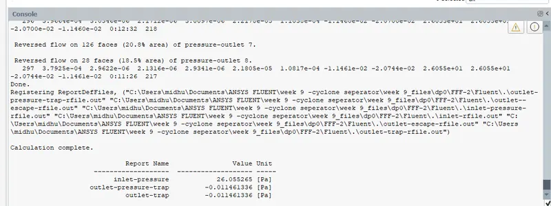
Pressure drop = 26.055-0.011 = 26.044 Pa
CASE 4: Inject velocity 5m/s and particle size is 5Micrometer
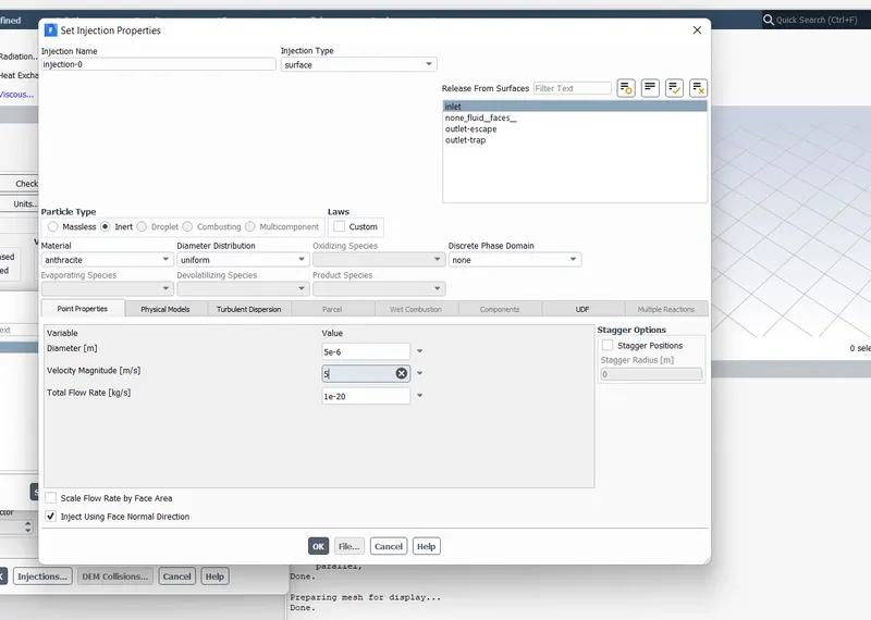
Giving Inject velocity 5m/s and particle size is 5Micrometer
RESULTS AND DISCUSSIONS:
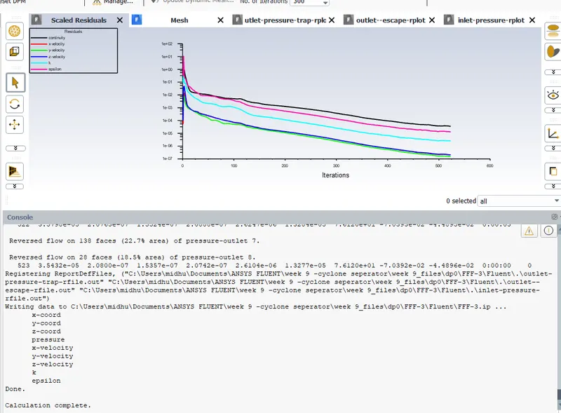
Showing residuals
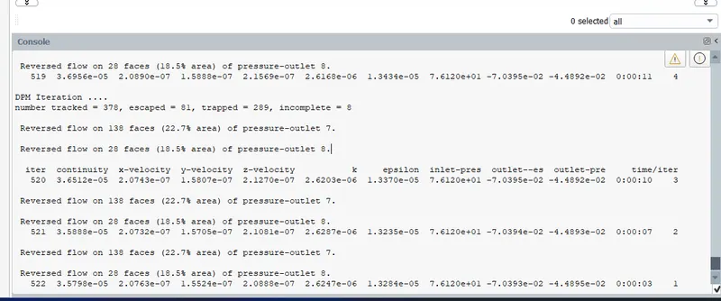
No of particles tracked = 378
No of particles trapped =289
No of particles escaped = 81
No of particles incomplete =8
Tracking efficiency = (289/378)X100=76.45%
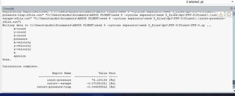
Pressure drop = 76.120-0.070 = 76.05 Pa
CASE 5: Inject velocity 1m/s and particle size 5Micrometer
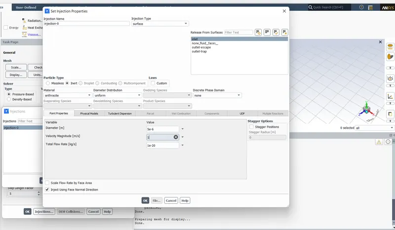
Giving inject velocity and particle size
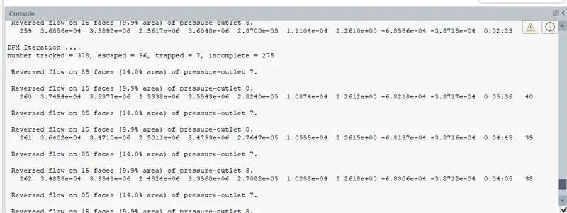
No of particles tracked = 378
No of particles trapped =7
No of particles escaped = 96
No of particles incomplete =275
Tracking efficiency = (7/378)X100=1.8%
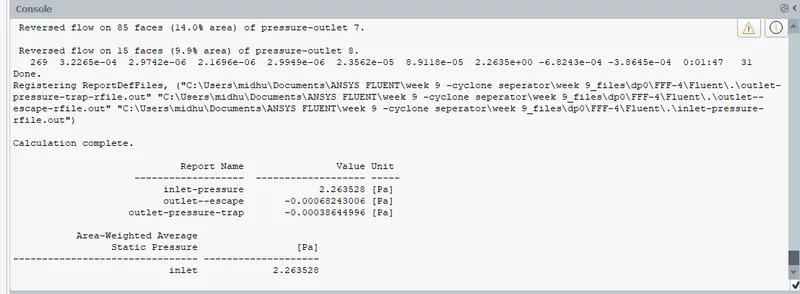
Pressure drop = 2.26-0.00068= 2.25Pa
CONCLUSIONS:
| Si No | Cases | Tracking Efficiency(%) | Pressure drop(Pa) | |
| (1) | 3m/s, 1Micrometer | 41 | 26.044 | |
| (2) | 3m/s, 3Micrometer | 58.46 | 26.092 | |
| (3) | 3m/s, 5Micrometer | 75.92 | 31.588 | |
| (4) | 5m/s, 5Micrometer | 76.45 | 76.05 | |
| (5) | 1m/s,5Micrometer | 1.81 | 2.25 | |
From this we can understand that when the size of particle increasing tracking efficiency also increasing and there is no much difference in the pressure drop.
When the velocity increasing trackin efficiency and pressure also increasing.