Week 8 - Simulating Cyclone separator with Discrete Phase Modelling

Cyclone separator:

Cyclonic separation is a means of separating different liquid phases (different liquid densities), or, separating
particles from a gas stream. Cyclone separators often form part of a pre-cleaning stage prior to a gas or liquid being discharged.

A cyclone separator has several colloquial names. These names include 'dust separator', 'dust collector, dust
extractor', 'cyclone extractor' and 'cyclone separator. Generally, smaller units are referred to as 'dust' separators or extractors, whilst large scale industrial separators are referred to as 'cyclone separators*
Gas cyclone separators are grouped into two main categories, reverse-flow and axial-flow.
In this project we use a reverse flow cyclone separator because this type of separator is the most common in use today.

Reverse flow cyclone separators are cone shaped.

Separate efficiency = No of particles trapped/No of particles tracked

Four empirical models used for cyclone separator efficiency:-

IOZIA AND LEITH MODEL
lozia and Leith (1990) logistic model is a modified version of Barth (1956) model which is developed based on force balance. The model assumes that a particle carried by the vortex endures the influence of two forces: a centrifugal force, and flow resistance. Core length zc, and core diameter dc, are given as: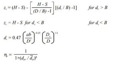

where dpc is 50% cut size given by Barth

• LI AND WANG MODEL
  This includes particle bounce or re-entrainment and turbulent diffusion at the cyclone wall. Li and Wang's
  model was developed based on the assumptions. An assumption made in this
  model is that the radial particle velocity and the radial concentration profile are not constant for uncollected particles within the cyclone. The concentration distribution is given by:

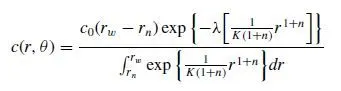
Where 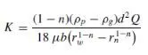and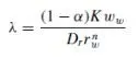

The efficiency is calculated from η = 1 - exp(-λθ1) where θ1=2π(S+L)/a

KOCH AND LICHT MODEL
This Model recognizes the inherently turbulent nature of cyclones and the distribution of gas residence times
within the cyclone. It describes particle motion in the entry and the collection regions with some assumptions,
1. The tangential velocity of particles is equal to the tangential velocity of the gas flow i.e. no slip' in tangential direction between the particle and the gas.
2. The tangential velocity is related to the radius of the cyclone by UR^n = constant
A force balance and the equation on this particles collection yield the grade efficiency.

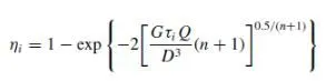
where

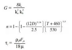
G is a factor related to the configuration of the cyclone, n is related to the vortex and τ is the relaxation term.

4. LAPPLE MODEL
It is a 1951 model developed by LAPPLE assuming that a particle entering a cyclone is evenly distributed along
with the inlet opening. It is based on Force Balance without considering the flow resistance. In this model, the
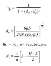
particle that travels from inlet half-width to the wall in the Cyclone is collected with 50% efficiency.
Efficiency,

Modeling approach :-

CAD clean up/Pre-process-SpaceClaim - Import the geometry which is given. Then extract the fluid volume.

Meshing :-Apply the elements size about and give the proper name selection.

Setup :- In this section, we set up the steady state simulation. Apply gravity in negative Y axis. kε - RNG - Swirl dominated flow model is applied for simulation. Apply Discrete phase, injections model. Applied boundary conditions. Initialize the simulation and apply certain no of iterations.

Solution :- we can see the animations of particle time and vortex core region.

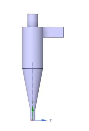
CAD modelling in SpaceClaim :-

Import the cyclone separator geometry which is provided into the SpaceClaim.

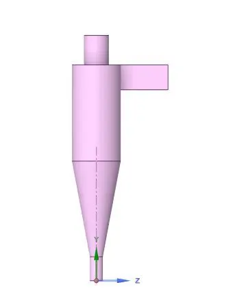
Extract the fluid volume from the cyclone separator. And supress the geometry for physics.

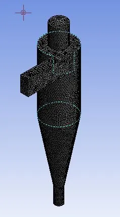
Meshing :-

Element size = 5 mm

No of elements = 574902

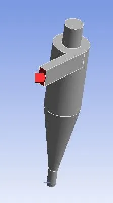
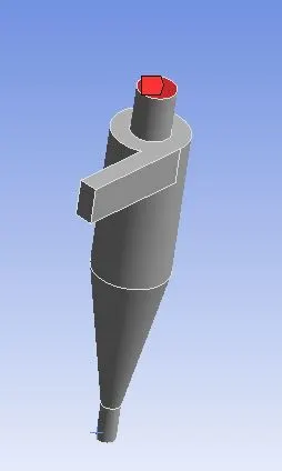
Apply name selections as inlet, outlet-1, outlet-2.

Inlet

Outlet-1

Outlet-2

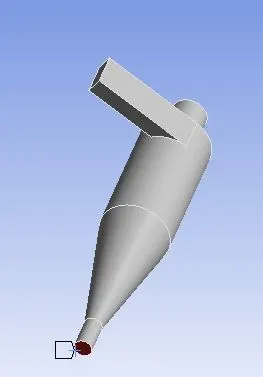
Objective ii)

inlet velocity = 3 m/s

a) particle diameter = 5 micrometer

Setup :- In this section, we set up the steady state simulation. Apply gravity in negative Y axis. kε - RNG - Swirl dominated flow model is applied for simulation.

Apply Discrete phase,

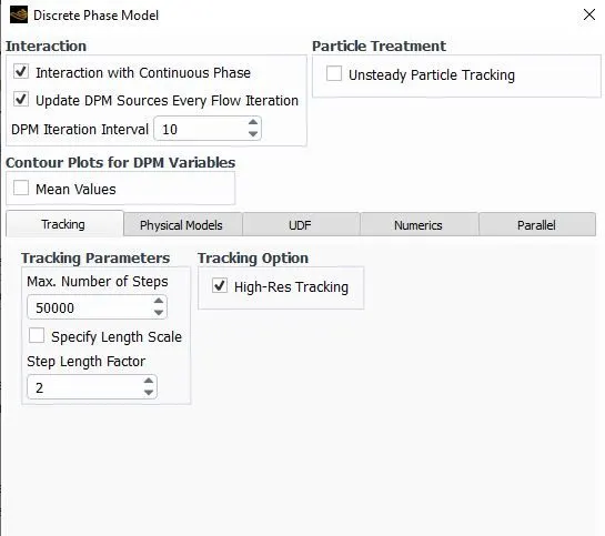
injections properties,

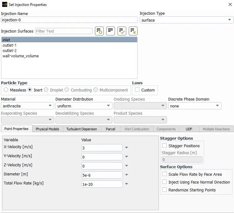
Applied boundary conditions. inlet velocity = 3 m/s , DPM = set discrete phase boundary type = reflect

For outlet -1 DPM = set discrete phase boundary type = escape

For outlet -2 DPM = set discrete phase boundary type = trap

Set method to 2nd oreder upwind for turbulance and dissipation.

Initialize the simulation and apply 600 iterations for simulation.

Then export the particle history data.

Solution :-

Residuals :-

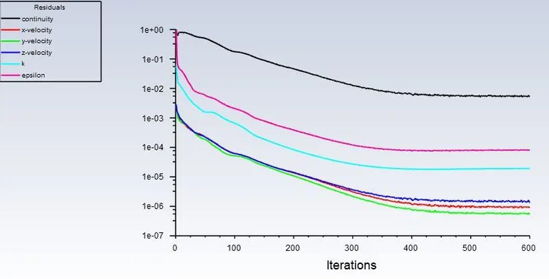
Result

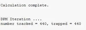
Number of particle tracked = 440

Number of particle trapped = 440

Number of particle escaped = 0

Results :-

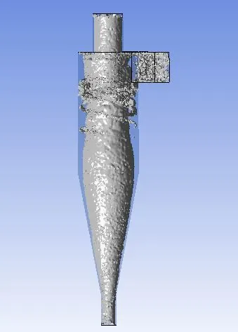
Vortex core region

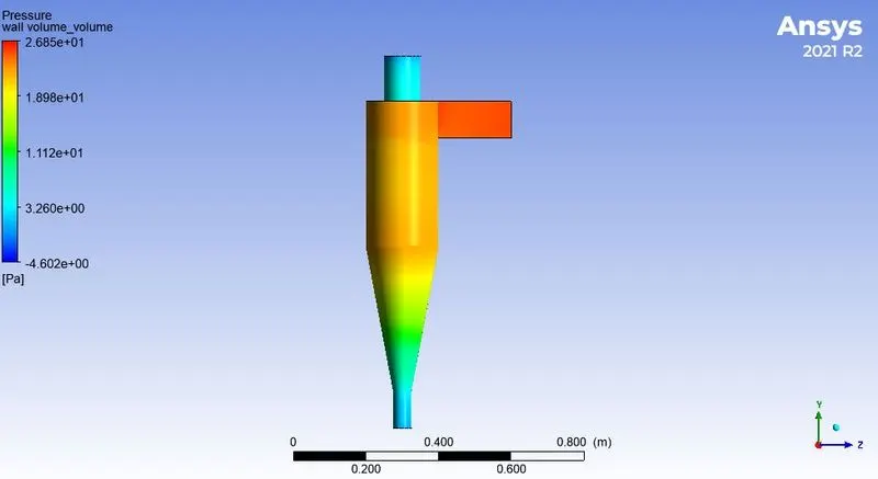
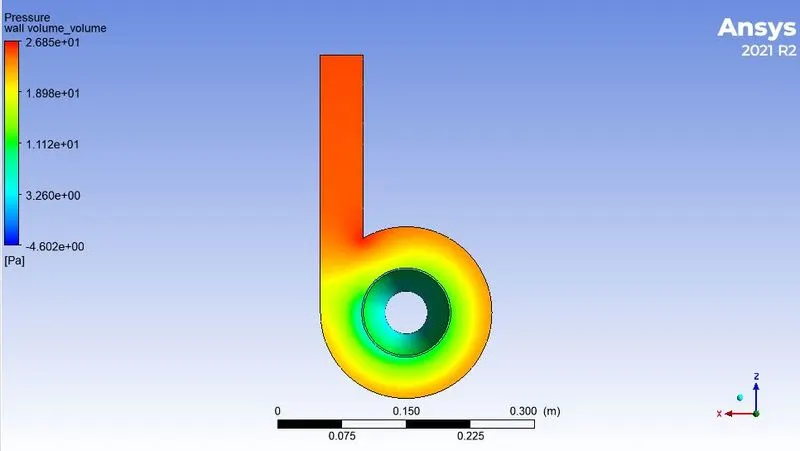
Pressure contour on the wall of the geometry

Anthracire particle time

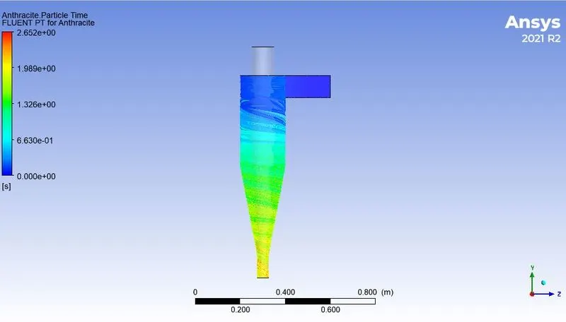
Animation :

https://drive.google.com/file/d/13Dsn8wysjSDchqH5d_KDBIc_84wmSuTi/view?usp=sharing

Separation efficiency = No of particles trapped/No of particles tracked

= 440/440

= 1

= 100%

b) particle diameter = 3 micrometer

Setup :- In this section, we set up the steady state simulation. Apply gravity in negative Y axis. kε - RNG - Swirl dominated flow model is applied for simulation.

Apply Discrete phase,

injections properties,

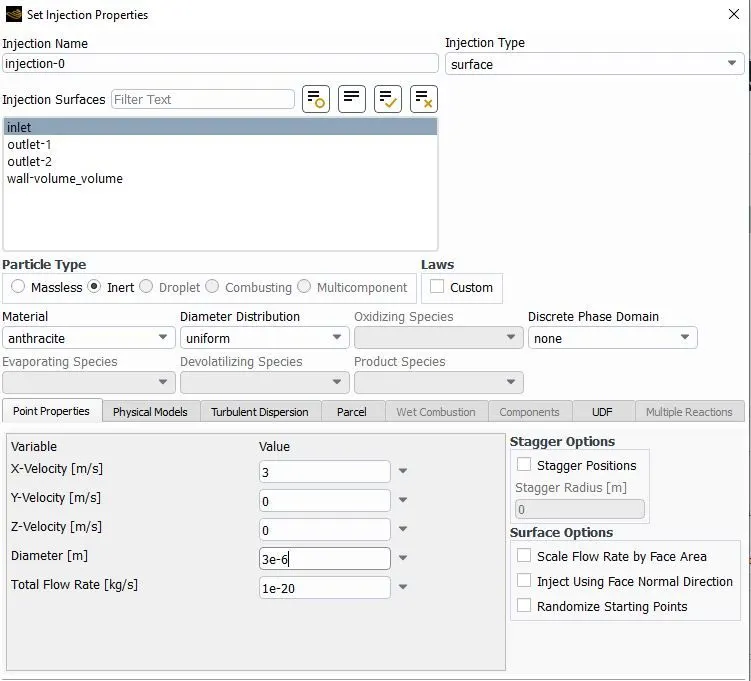
Applied boundary conditions. inlet velocity = 3 m/s , DPM = set discrete phase boundary type = reflect

For outlet -1 DPM = set discrete phase boundary type = escape

For outlet -2 DPM = set discrete phase boundary type = trap

Set method to 2nd oreder upwind for turbulance and dissipation.

Initialize the simulation and apply 600 iterations for simulation.

Then export the particle history data.

Solution :-

Residuals :-

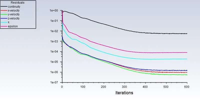
Result

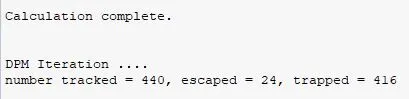
Number of particle tracked = 440

Number of particle trapped = 416

Number of particle escaped = 24

Results :-

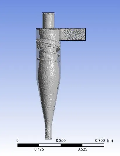
Vortex core region

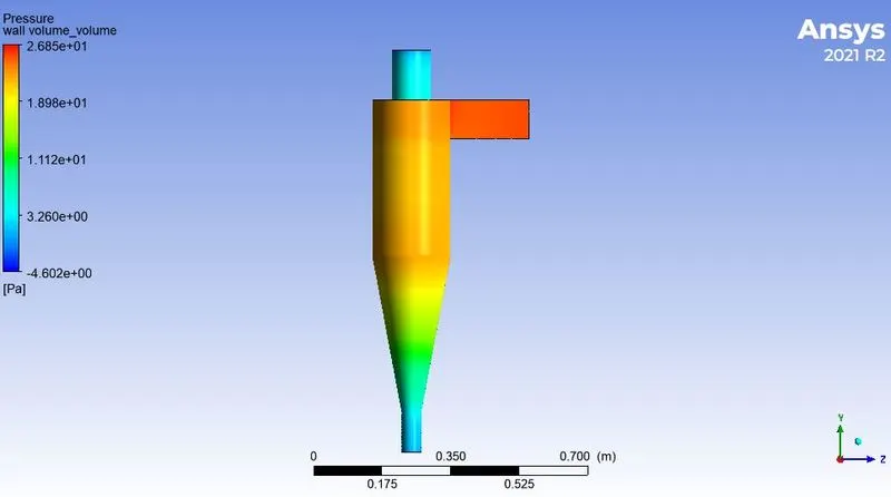
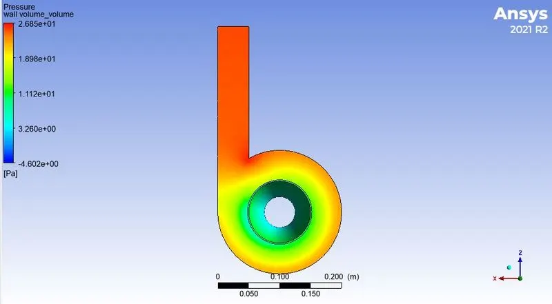
Pressure contour on the wall of the geometry

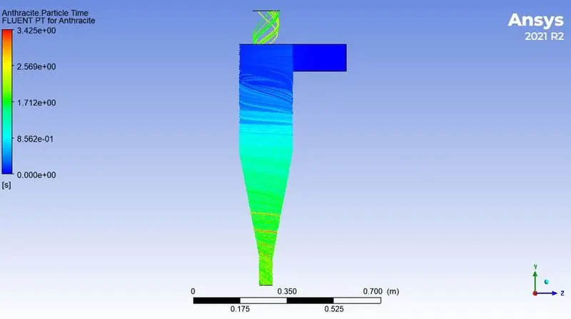
Anthracire particle time

Animation :

https://drive.google.com/file/d/1VG1z9PILMu8vR5qStj7C2NUu6Zw9EhJh/view?usp=sharing

Separation efficiency = No of particles trapped/No of particles tracked

= 416/440

= 0.945

= 94.5%

b) particle diameter = 1 micrometer

Setup :- In this section, we set up the steady state simulation. Apply gravity in negative Y axis. kε - RNG - Swirl dominated flow model is applied for simulation.

Apply Discrete phase,

injections properties,

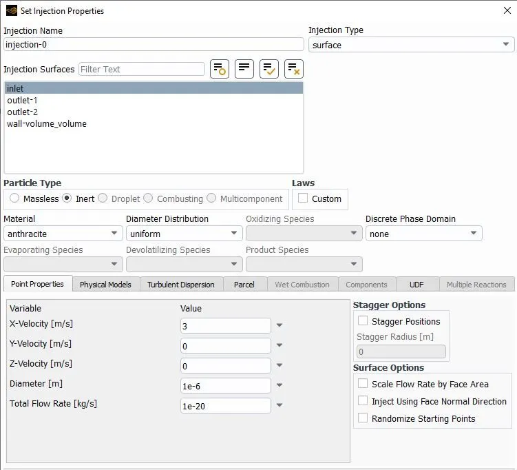
Applied boundary conditions. inlet velocity = 3 m/s , DPM = set discrete phase boundary type = reflect

For outlet -1 DPM = set discrete phase boundary type = escape

For outlet -2 DPM = set discrete phase boundary type = trap

Set method to 2nd oreder upwind for turbulance and dissipation.

Initialize the simulation and apply 600 iterations for simulation.

Then export the particle history data.

Solution :-

Residuals :-

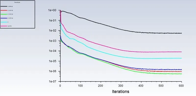
Result

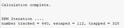
Number of particle tracked = 440

Number of particle trapped = 328

Number of particle escaped = 112

Results :-

Vortex core region

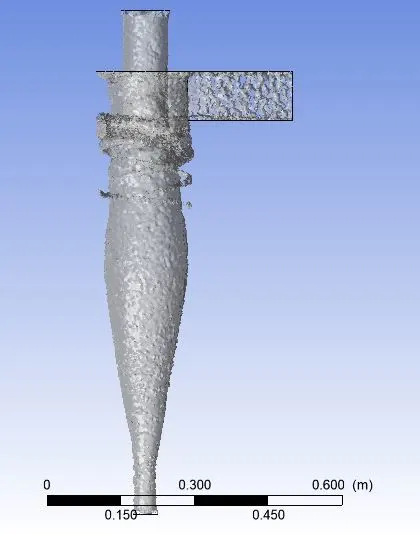
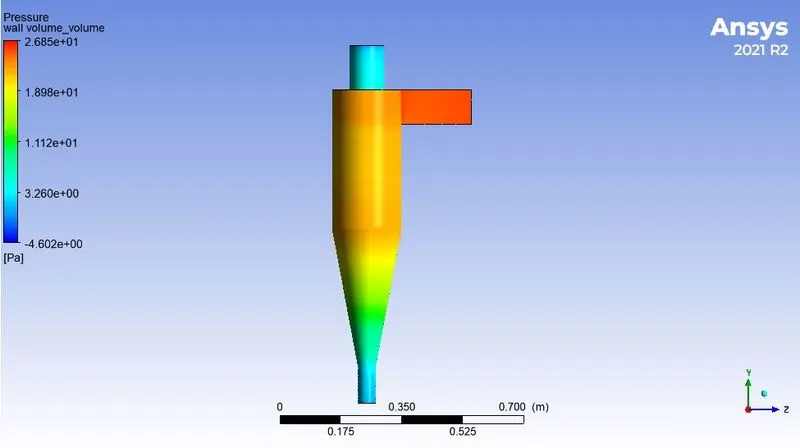
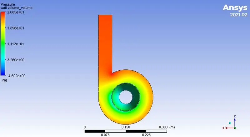
Pressure contour on the wall of the geometry

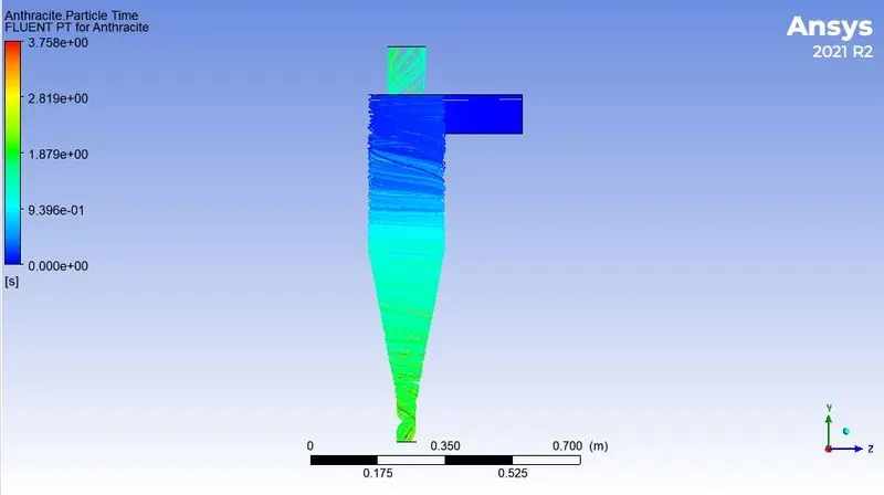
Anthracire particle time

Animation :

https://drive.google.com/file/d/1hjg2Bzd9VQchaF5AqQ5QalsvINMZLaUy/view?usp=sharing

Separation efficiency = No of particles trapped/No of particles tracked

= 328/440

= 0.745

= 74.5%

velocity at inlet (m/s)	Particle diameter (μm)	No of particle tracked	No of particle trapped	No of particle escaped	Separation efficiency(%)
3 m/s	5 μm	440	440	0	100 %
3 m/s	3 μm	440	416	24	94.5 %
3 m/s	1 μm	440	328	112	74.5 %

Ae per the above table we can see that if we varying the diameter of the particles by keeping inlet velocity as constant, as the diameter of the particles increase the number of particles which are getting trapped at outlet-2 (lower outlet) increase and the number of particles which are getting escaped decrease. From the formula of the separation efficiency no of particles which are trapped increase the separation efficiency also increases. So diameter of the particles increase efficiency will be increased.

Objective - ii)

Diameter of particle = 5 micrometer

a) Inlet velocity = 1 m/s

Setup :- In this section, we set up the steady state simulation. Apply gravity in negative Y axis. kε - RNG - Swirl dominated flow model is applied for simulation.

Apply Discrete phase,

injections properties,

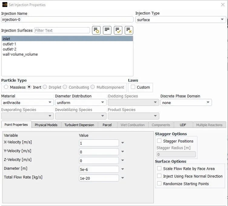
Applied boundary conditions. inlet velocity = 1 m/s , DPM = set discrete phase boundary type = reflect

For outlet -1 DPM = set discrete phase boundary type = escape

For outlet -2 DPM = set discrete phase boundary type = trap

Set method to 2nd oreder upwind for turbulance and dissipation.

Initialize the simulation and apply 600 iterations for simulation.

Then export the particle history data.

Solution :-

Residuals :-

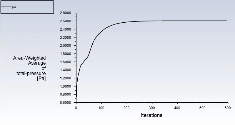
Total Pressure at inlet = 2.605 Pa

Total pressure at outlet-2 = 0.2358 Pa

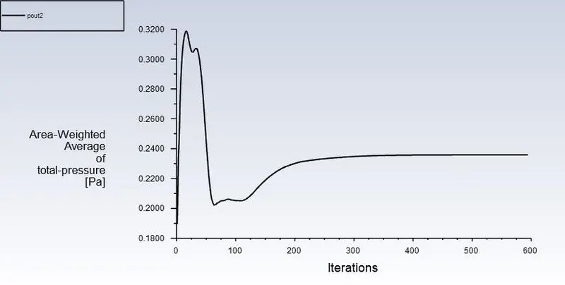
Pressure drop = 2.605 - 0.2358 = 2.3692 Pa

Result

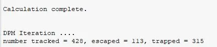
Number of particle tracked = 428

Number of particle trapped = 315

Number of particle escaped = 113

Results :-

Vortex core region

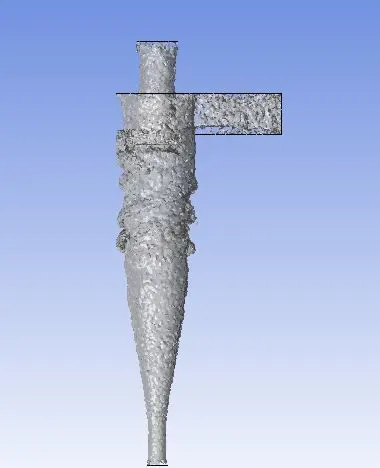
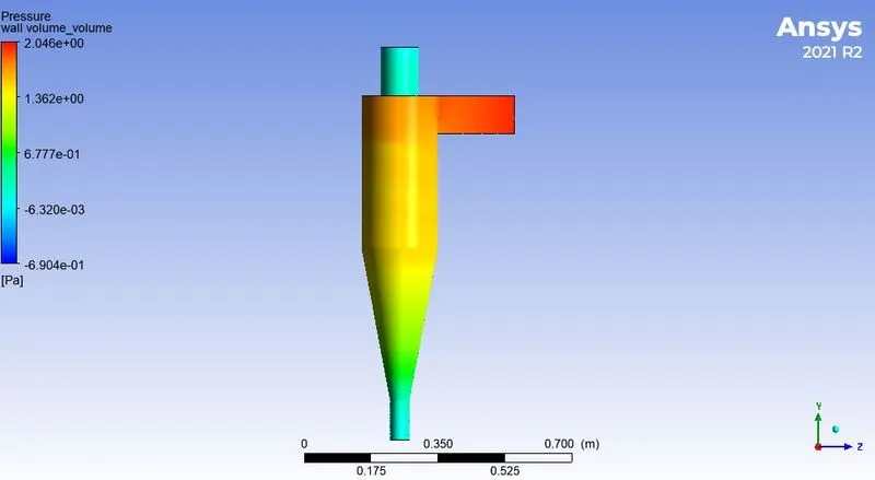
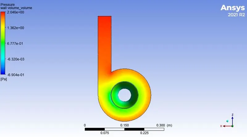
Pressure contour on the wall of the geometry

Anthracire particle time

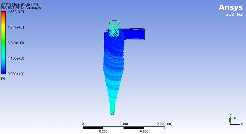
Animation :

https://drive.google.com/file/d/1XillzM08Jn2S8tJrp4ESTiD4qsoUW9fl/view?usp=sharing

Separation efficiency = No of particles trapped/No of particles tracked

= 315/428

= 0.7359

= 73.59 %

b) inlet velocity = 3 m/s

( As we have done in previous objective)

Setup :- In this section, we set up the steady state simulation. Apply gravity in negative Y axis. kε - RNG - Swirl dominated flow model is applied for simulation.

Apply Discrete phase,

injections properties,

Applied boundary conditions. inlet velocity = 3 m/s , DPM = set discrete phase boundary type = reflect

For outlet -1 DPM = set discrete phase boundary type = escape

For outlet -2 DPM = set discrete phase boundary type = trap

Set method to 2nd oreder upwind for turbulance and dissipation.

Initialize the simulation and apply 600 iterations for simulation.

Then export the particle history data.

Solution :-

Residuals :-

Total Pressure at inlet = 30.7774 Pa

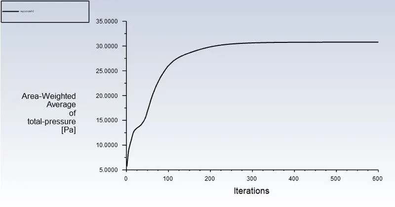
Total pressure at outlet-2 = 2.1411 Pa

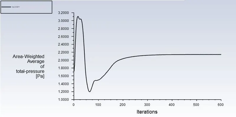
Pressure drop = 30.7774 - 2.1411 = 28.6363 Pa

Result

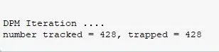
Number of particle tracked = 428

Number of particle trapped = 428

Number of particle escaped = 0

Results :-

Vortex core region

Pressure contour on the wall of the geometry

Anthracire particle time

Animation :

https://drive.google.com/file/d/13Dsn8wysjSDchqH5d_KDBIc_84wmSuTi/view?usp=sharing

Separation efficiency = No of particles trapped/No of particles tracked

= 428/428

= 1

= 100%

c) inlet velocity = 5 m/s

Setup :- In this section, we set up the steady state simulation. Apply gravity in negative Y axis. kε - RNG - Swirl dominated flow model is applied for simulation.

Apply Discrete phase,

injections properties,

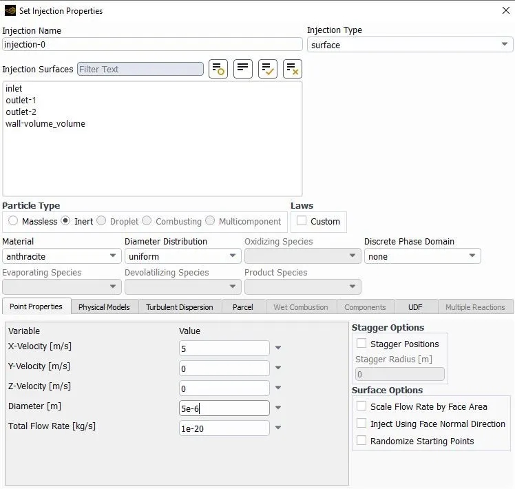
Applied boundary conditions. inlet velocity = 5 m/s , DPM = set discrete phase boundary type = reflect

For outlet -1 DPM = set discrete phase boundary type = escape

For outlet -2 DPM = set discrete phase boundary type = trap

Set method to 2nd oreder upwind for turbulance and dissipation.

Initialize the simulation and apply 600 iterations for simulation.

Then export the particle history data.

Solution :-

Residuals :-

Total pressure at inlet = 88.5155 Pa

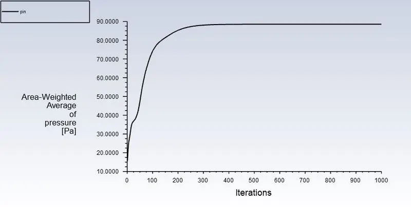
Total pressure at outlet-2 = 6.0962 Pa

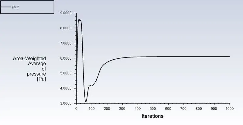
Total pressure drop = 88.5155 - 6.0962 = 82.4193 Pa

Result

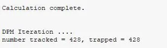
Number of particle tracked = 428

Number of particle trapped = 428

Number of particle escaped = 0

Results :-

Vortex core region

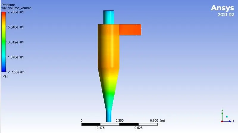
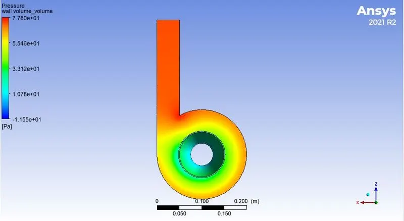
Pressure contour on the wall of the geometry

Anthracire particle time

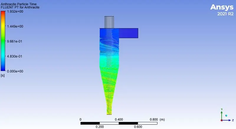
Animation :

https://drive.google.com/file/d/11ssFUcv19K9wYLl_7m5or-QQoPW1Sg-j/view?usp=sharing

Separation efficiency = No of particles trapped/No of particles tracked

= 426/426

= 1

= 100%

Particle diameter (μm)	Velocity at inlet (m/s)	No of particle tracked	No of particle trapped	No of particle escaped	Separation efficiency(%)	Pressure drop (Pa)
5 μm	1 m/s	428	315	113	73.59 %	2.3692
5 μm	3 m/s	428	428	0	100%	28.6363
5 μm	5 m/s	428	428	0	100 %	82.4193

Ae per the above table we can see that if we varying the inlet velocity by keeping diameter of particles as constant, as the inlet velocity increase the number of particles which are getting trapped at outlet-2 (lower outlet) increase and the number of particles which are getting escaped decrease. From the formula of the separation efficiency no of particles which are trapped increase the separation efficiency also increases. So inlet velocity increase efficiency will be increased. And we can see the that the pressure drop also increases drastically by increasing the inlet velocity.

CONCLUSION:

The Discrete Phase Model (DPM) is used in the simulation of the mixture of air (continuous phase) and Anthracite particles (discrete phase) through a cyclone separator. The Anthracite particles are separated from the mixture by the separator. The Anthracite particles are tracked and their trajectories are estimated. The separation efficiency is calculated by varying the diameter of the particles as well as varying the velocities. It is found that separation efficiency decreases with a decrease in the diameter of the particle and the separation efficiency increases with an increase in velocity at the inlet. But with an increase in efficiency, the total pressure drop across the system increases drastically as well.