Week 3.5 - Deriving 4th order approximation of a 2nd order derivative using Taylor Table method
1.Central difference:-To derive central difference for fourth order approximation of second order derivative by Taylor table method of finite difference method by using equation given below.
∂2f/∂x2 = a*f(i-2)+b*f(i-1)+c*f(i)+d*f(i+1)+e*f(i+2)
Taylor table for central difference of fourth order approximation-
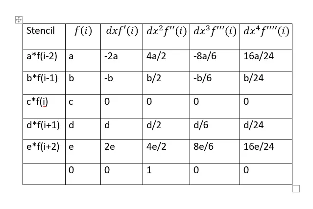
Following MATLAB code is used to find the co-efficients-
% find the co-efficients for central difference scheme
A=[1 1 1 1 1;-2 -1 0 1 2;4/2 1/2 0 1/2 4/2;-8/6 -1/6 0 1/6 8/6;16/24 1/24 0 1/24 16/24];
B=[0;0;1;0;0];

X = inv(A)*B
output- a=-0.0833
b=1.3333
c=-2.5000
d=1.3333
e=-0.0833
MATLAB code- In this program,we have compute absolute error which is basically the difference of Central
difference and second order analytical derivative and then by using function out we are calling this function in the main program to compare with other schemes.
% function for 4th order approximatin for second order derivative using
% central difference
function out=central_difference_error(x,dx)
%Function=exp(x) *cos(x)

%Analytical derivative
%second order analytical derivative
analytical_derivative =-2*sin(x)*exp(x);

%Numerical derivative
%Fourth order approximation
central_difference=(-0.0833*exp(x-2*dx)*cos(x-2*dx) +1.3333*exp(x-dx)*cos(x-dx)-2.50*exp(x)*cos(x)+1.3333*exp(x+dx)*cos(x+dx)-0.0833*exp(x+2*dx)*cos(x+2*dx))/dx^2;
out=abs(central_difference-analytical_derivative);
end
2.Skewed right side difference - To derive skewed right side difference for fourth order approximation of second order derivative by Taylor table method of finite difference method by using equation given below.
∂2f/∂x2 = a*f(i)+b*f(i+1)+c*f(i+2)+d*f(i+3)+e*f(i+4)
Taylor table for skewed right sided difference of fourth order approximation-
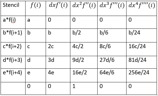
Following MATLAB code is used to find the co-efficients-
% find the co-efficients for skewed right side difference scheme

A=[1 1 1 1 1;0 1 2 3 4;0 1/2 4/2 9/2 16/2;0 1/6 8/6 27/6 64/6;0 1/24 16/24 81/24 256/24];
B=[0;0;1;0;0];

X=inv(A)*B
output- a=2.9167
b=-8.6667
c=9.5000
d=-4.6667
e=0.9167
MATLAB code- In this program,we have compute absolute error which is basically the difference of skewed right side difference and second order analytical derivative and then by using function out we are calling this function in the main program to compare with other schemes.
% function for 4th order approximatin for second order derivative using
% skewed right side difference
function out=skewed_right_side_error(x,dx)
%Function=exp(x)*cos(x)

%Analytical derivative
%second order analytical derivative
analytical_derivative =-2*sin(x)*exp(x);

%Numerical derivative
%Fourth order approximation
skewed_right_side_difference=(2.9167*exp(x)*cos(x)-8:6667*exp(x+dx)*cos(x+dx)+9.500*exp(x+2*dx)*cos(x+2*dx)-4.667*exp(x+3*dx)*cos(x+3*dx)+0.9167*exp(x+4*dx)*cos(x+4*dx))/(dx^2);
out=abs(skewed_right_side_difference-analytical_derivative);
end
3.Skewed left side difference:-To derive skewed left side difference for fourth order approximation of second order
lerivative by Taylor table method of finite difference method by using equation given below
∂2f/∂x2= a*f(i)+b*f(i-1)+c*f(i-2)+d*f(i-3)+e*f(i-4)
Taylor table for skewed left sided difference of fourth order approximation-
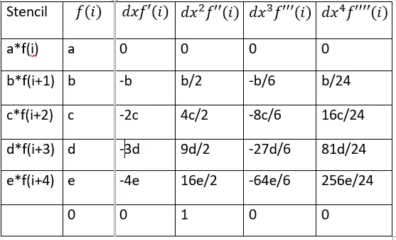
Following MATLAB code is used to find the co-efficients-
% find the co-efficients for skewed left side difference scheme
A=[1 1 1 1 1;0 -1 -2 -3 -4;0 1/2 4/2 9/2 16/2;0 -1/6 -8/6 -27/6 -64/6;0 1/24 16/24 81/24 256/24];
B=[0;0;1;0;0];

X=inv(A)*B
output- a=2.9167
b=-8.6667
c=9.5000
d=-4.6667
e=0.9167
MATLAB code- In this program,we have compute absolute error which is basically the difference of skewed right side difference and second order analytical derivative and then by using function out we are calling this function in the main program to compare with other schemes.
% function for 4th order approximatin for second order derivative using
% skewed left side difference
function out=skewed_left_side_error(x,dx)
%Function=exp(x)*cos(x)

%Analytical derivative
%second order analytical derivative
analytical_derivative =-2*sin(x)*exp(x);

%Numerical derivative
%Fourth order approximation
skewed_left_side_difference=(2.9167*exp(x)*cos(x)-8:6667*exp(x+dx)*cos(x+dx)+9.500*exp(x+2*dx)*cos(x+2*dx)-4.667*exp(x+3*dx)*cos(x+3*dx)+0.9167*exp(x+4*dx)*cos(x+4*dx))/(dx^2);
out=abs(skewed_left_side_difference-analytical_derivative);
end
The order of accuracy:-
For central scheme- The order of accuracy P , No of nodes in the stencil N=5 , Order of derivative Q = 2
P = N - Q+1 = 5 - 2+1
P = 4
For skewed scheme - The order of accuracy P , No of nodes in the stencil N=5 , Order of derivative Q = 2
P = N - Q = 5 - 2
P = 3
From the above values of P , it's proven that central schemes are more accurate than skewed schemes.
MAIN PROGRAM:- In this program we have called all above schemes program to compare each other at the same value
of x and range of dx.And to see which scheme gives less error.
% comparision of central_difference_error, skewed_right_side_error, skewed_left_side_error

% input parameter
x=pi/3;
dx=linspace(pi/4,pi/4000,80);

%Function=exp(x)*cos(x)

%Analytical derivative
%second order analytical derivative
analytical_derivative =-2*sin(x)*exp(x);

%For loop;
for i=1:length(dx)
central_difference_error(i)=central_difference(x,dx(i));
skewed_right_side_error(i) =skewed_right_side(x,dx(i));
skewed_left_side_error(i)=skewed_left_side(x,dx(i));
end

%plotting;
figure
loglog(dx,central_difference_error,'r')
hold on
loglog(dx,skewed_righ_side_error,'g')
hold on
loglog(dx,skewed_left_side_error,'b')

%Label
xlabel('dx')
ylabel('error')
legend('central difference error','skewed right side error','skewed left side error')
By observing above plot we can conclude following observation which are as follows
-Skewed right gives maximum error or in otherwords we can say that its unstable as compared to other scheme.
- Central diference gives lowest error or in otherwords we can say that its stable as compared to other scheme.
- Skewed left gives error somewhere in between skewed right difference and central diference.
Now,Although central difference gives less error as compared to skewed right and left side difference,but in some
cases skewed difference scheme is more useful as compared to central difference. To learn in detail let see an
example.
- If we want calculate error at boundary,we cannot apply central diference sheme since it require value from
both end so,in this case we can apply skewed diference scheme
Also,we can calculate error at boundary by using forward difference scheme or backward difference
scheme,but it wont be good decision because FDS and BDS has low order of approximation so it would be have
more error.Therefore,skewed difference scheme is prefer for such case.