Week 5.1 - Mid term project - Solving the steady and unsteady 2D heat conduction problem
- For Steady State Flow:
The generalised 2D temperature Equation is,
∂2T/∂x2+∂2T/∂y2=0
We discretize the equestion by central differencing,
The Eqn with respect to X becomes,
∂2T/∂x2=(T(i-1,j)-2T(i,j)+T(i+1,j))/Δx^2
• The Eqn with respect to Y becomes,
∂2T/∂y2= (T(i,j-1)-2T(i,j)+T(i,j+1))/Δy^2
Since we assumed nx=ny then we can take Δx^2=Δy^2
then the Eqn becomes as
T(i, j) = (T(i-1,j)+T(i+1,j)+T(i,j-1)+T(i,j+1))/4
% Script for solving 2d Steady state heat conduction eqn

% Inputs
L=1; %length of domain is a unit square
%no of grid points along X & Y
nx=30;
ny=nx;
x=linspace(0, L,nx);
y=linspace(0,L,ny) ;
dx=x(2)-x(1);
dy=y(2)-y(1) ;
error = 9e9;
tol = le-4;
alpha=1.8;%For SOR
%Defining boundary conditions
T_L = 400;
T_T = 600;
T_R = 800;
T_B = 900;
T = ones(nx, ny) ;
T(2:ny-1,1) = T_L;
T(2:ny-1,nx) = T_R;
T(1,2:nx-1) = T_T;
T(nx,2:ny-1) = T_B;

% calculating average temperature at the matrix corners
T(1,1) =. (T_T + T_L)/2;
T (nx, ny) = (T_R + T_B) /2;
T (1,ny) =(T_T+T_R)/2;
T(nx,1) = (T_L + T_B)/2;
% other factors to be considered
[X,Y] = meshgrid(x,y);
Told = T;
%Calculation of 2d Steady state heat conduction eqn
iterative_solver=1:3;
% Jacobi Iteration
for iterative_solver=1
tic;
if iterative_solver==1
jacobi_iter=1;
while(error > tol)
for i=2:nx-1
for j=2:ny-1
T(i,j) = 0.25*(Told(i-1,j)+Told(i+1,j)+Told(i,j-1)+Told(i,j+1)) ;
end
end

error = max(max(abs(Told-T)));
Told = T;
jacobi_iter=jacobi_iter+1;
end
end
F=toc;

%plot
figure(1)

[M, N]=contourf(X, Y, T) ;
clabel(M,N)
colormap(jet)
colorbar
title_text=sprintf('Jacobi Steady iteration number =%d , Total Time F=%fs', jacobi_iter, F) ;
title(title_text)
xlabel('X-axis')
ylabel('Y-axis')
fprintf('No of Iteration in jacobi=%dn',jacobi_iter);
end

% GS Iter
for iterative_solver=2
%update values
L=1;
nx=30;
ny=nx;
x=linspace(0, L, nx) ;
y=linspace(0, L, ny) ;
dx=x(2)-x(1) ;
dy= y(2)-y(1);
error = 9e9;
tol = le-4;
T_L = 400;
T_T = 600;
T_R = 800;
T_B=900;
T=ones(nx, ny) ;
T(2:ny-1,1) = T_L;
T(2:ny-1, nx)= T_R;
T(1,2:nx-1) = T_T;
T(nx,2:ny-1)=T_B;
T (1,1) = (T_T + T_L)/2;
T(nx, ny) = (T_R + T_B) /2;
T (1, ny) = (T_T + T_R)/2;
T(nx,1)= (T_L + T_B)/2;

[X, Y] = meshgrid(x,y);
Told = T;
tic;

if iterative_solver==2
GS_iter=1;
while(error > tol)
for i=2: nx-1
for j=2:ny-1
T(i,j) = 0.25*(T(i-1,j) +Told(i+1,j)+T(i,j-1)+Told (i,j+1));
end
end
error = max(max(abs(Told-T)));
Told = T;
GS_iter=GS_iter+1;
end
end

 F=toc;
% plot
figure(2)
[M, N] =contourf (X, Y, T);
clabel(M,N)
colormap(jet)
colorbar
title_text=sprintf('GS steady iteration number =%d , Total Time F=%Fs',GS_iter,F);
title(title_text)
xlabel('X-axis')
ylabel('Y-axis')
fprintf ('No of Iteration in GS=%dn',GS_iter);
end

%S0R Iter
for iterative_solver=3
%update values
L=1;
nx=30;
ny=nx;
x=iinspace(0,L, nx);
y=linspace(0,L, ny) ;
dx=x(2)-x(1) ;
dy=y(2) -y(1) ;
error = 9e9;
 tol = le-4;
T_L = 400;
T_T = 600;
T_R = 800;
T_B = 900;
T=ones(nx,ny);
T(2:ny-1,1) = T_L;
T(2:ny-1,nx) = T_R;
T(1,2:nx-1) = T_T;
T(nx,2:ny-1)= T_B;
T(1,1) = (T_T + T_L)/2;
T(nx, ny) = (T_R + T_B)/2;
T (1,ny) = (T_T + T_R)/2;
T (nx,1) = (T_L + T_B)/2;
[X,Y] = meshgrid(x,y) ;
Told = T;
tic;
if iterative_solver==3
SOR_iter=1;
while(error > tol)
for i=2:nx-1
for j=2:ny-1
T(i,j) = ((1-alpha)* Told(i,j)+(alpha*0.25*(T(i,j-1)+Told(i,j+1)+T(i-,j)+Told(1+1,j))));
end
end
error = max(ma (abs(Told-T)));
 Told = T;
SOR_iter=SOR_iter+1;
end
end

F=toc:
% plot
figure(3)
[M,N]=contourf(X,Y, T);
clabel(M,N)
colormap(jet)
colorbar
title_text=sprintf('SOR steady iteration number =%d ,Total Time F=%fs',SOR_iter,F);
title(title_ text)
xlabel('X-axis')
ylabel('Y-axis')
fprintf ('No of Iteration in SOR=%dn',SOR_iter);
end
Solving through Jacobi, Gauss-Seidel (GS) & Successive Over Relaxation (SOR) Iteration method:
Steady state program output:-
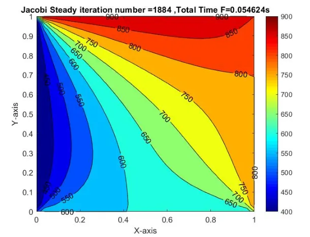
1. Jacobi steady iteration
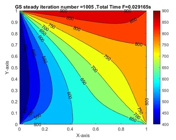
2. GS steady iteration
3. SOR steady iteration
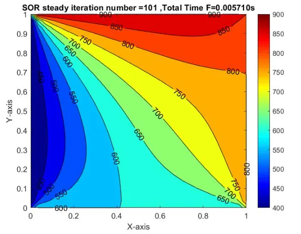
As from stated on the figure, the number of iteration required to converge the solution is more in Jacobi iteration
scheme followed by Gauss Siedle iteraion and SR scheme. Which obviously means the computaional time required
for a computer program to run the iteration is more in Jacobi followed by GS and SOR scheme.
- For Unteady State Flow:
The generalised 2D temperature Equation is,
α(∂2T/∂x2+∂2T/∂y2)=∂T/∂t
We discretize the equestion by central differencing and time gradient eq with forward differencing method
The Eqn with respect to X becomes,
∂2T/∂x2=(T(i-1,j)-2T(i,j)+T(i+1,j))/Δx^2
• The Eqn with respect to Y becomes,
∂2T/∂y2= (T(i,j-1)-2T(i,j)+T(i,j+1))/Δy^2
The Eqn with respect to Time becomes,
∂T/∂t=(T^n+1(i,j)-T^n(i,j))/Δt
We define two constant namely k1 and k2
k1=αΔt/Δx^2
k2=αΔt/Δy^2
- Solving Transient Flow(Explicit):
%Script for solving 2d Transient state heat conduction eqn (Explicit)

%Inputs
L=1; %length of domain is a unit square
%no of grid points along X & Y
nx=30;
ny=nx;
x=linspace(0,L, nx) ;
y=linspace(0, L, ny) ;
dx=x(2)-x(1);
dy= y(2)-y(1);
error = 9e9;
tol = le-4;
dt=0.01;
alpha=1.88e-5;%thermal diffusivity for steel
%Defining boundary conditions
T_L = 400;
T_T = 600;
T_R = 800;
T_B = 900;
T = ones(nx,ny);
T (2: ny-1, 1) = T_L;
T (2:ny-1, nx) = T_R;
T (1,2:nx-1)= T_T;
T(nx,2:ny-1) = T_B;

%% calculating average temperature at the matrix corners
T (1,1) = (T_T + T_L)/2;
T(nx, ny) = (T_R + T_B)/2;
T (1,ny) = (T_T + T_R)/2;
T(nx,1) = (T_L + T_B)/2;

%other factors to be considered
%we know the values for constants k
k1 = (alpha*dt)/(dx^2);
k2 = (alpha"dt)/(dy^2);
[X,Y] = meshgrid(x,y);
Told = T:
%% Calculation of 2d Transient state heat conduction eq in Explicit
iterative_solver=1;
tic;

if iterative_solver==1
solver_counter=1;
while(error > tol)
for i=2:nx-1
for j=2:ny -1
terml = Told(i,j);
term2 = k1*(Told(i+1,j)-2*Told(i,j)+Told(i-1,j));
term3 = k2*(Told(i,j+1)-2*Told(i,j)+Told(i,j-1));
T(i,j) = term1+term2+term3;
end
end
error = max(max(abs(Told-T)));
Told = T;
solver_counter=solver_counter+1;
end
end
F=toc;

% plot
figure(1)
[M,N]=contourf(x, Y,T);
clabel(M,N)
colormap(jet)
colorbar
title_text=sprintf('Transient iteration number through explicit=%d ,Total Time F=%fs',solver_counter, F);
title(title_text)
xlabel('X-axis')
ylabel('Y-axis')
fprintf('No of Iteration in Transient (explicit)=%dn',solver_counter);
end
Transient flow (Explicit) output:-
Transient iteration through explicit
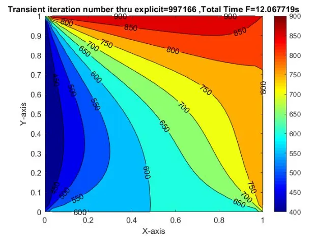
For Explicit Scheme, we cannot use the same time steps and length of mesh domain, as it yeids to higher CFL
number, which leads to unstable solution unconverging. For the convenient I have taken the time steps and length
domain for both x and y axis mentioned in the code section.
- Solving transient flow (Implicit) by Jacobi, GS and SOR
% Script for solving 2d Transient state heat conduction eqn (Implicit)
%Inputs
L=1;n%length of domain is a unit square
%no of grid points along X & Y
nx=30;
ny=nx;
x=linspace(0,L,nx);
y=linspace(0,L,ny);
dx=x(2)-x(1);
dy=y(2)-y(1) ;
error =9e9;
tol=1e-4;
dt = 2000;
alpha=1.88e-5;%thermal diffusivity for steel
alpha1=1.8;%For SOR

%Defining boundary conditions
T_L = 400;
T_T = 600;
T_R = 800;
T_B = 900;
T = ones(nx,ny);
T(2:ny-1,1) = T_L;
T(2:ny-1,nx)= T_R;
T(1,2:nx-1) = T_T;
T(nx,2:ny-1)= T_B;

% calculating average temperature at the matrix corners
T(1,1) = (T_T + T_L)/2;
T(nx, ny) = (T_R + T_B)/2;
T(1, ny)= (T_T + T_R) /2;
T(nx,1) = (T_L + T_B)/2;

%other factors to be considered
%we know the values for constants k
k1 = (alpha*dt)/(dx^2);
k2 = (alpha*dt)/(dy^2);
[X,Y] = meshgrid(x,y);
Told = T;
T_Prev_dt = Told;

%Calculation of 2d Transient state heat conduction eqn(Implicit)
iterative_solver=1:3;
%% Jacobi Iteration
term1=(1+2*k1+2*k2)^(-1);
term2=k1*term1;
term3=k2*term1;
for iterative_solver=1
tic;
if iterative_solver==1
jacobi_iter=1;
while (error > tol)
for i=2:nx-1
for j=2:ny-1
 H = (Told(i-1,j)+Told(i+1,j));
V = (Told(i,j-1)+Told(i,j+1));
T(i,j) = term1*T _Prev_dt(i,j)+term2*H+term3*V;
end
end

error = max(max(abs(Told-T)));
Told = T;
jacobi_iter=jacobiiter+1;
end
end
F=toc;

%plot
figure(1)
[M,N]=contourf(X, Y, T);
clabel(M,N)
colormap(jet)
colorbar
title_text=sprintf('Jacobi UnSteady (Implicit) iteration number =%d ,Total Time F=fs',jacobi_iter,F);
title(title _text)
xlabel('X-axis')
ylabel ('Y-axis')
fprintf('No of Iteration in jacobi=%dn',jacobi_iter);
end

% GS Iter
%update values
L=1;
nx=30;
ny=nx;
x=linspace(0,L,nx);
y=linspace(0,L,ny);
dx=x(2) -x(1);
dy= y(2)-y(1);
error = 9e9;
tol = 1e-4;
dt=2000;
alpha=1.88e-5; %thermal diffusivity for steel
T_L = 400;
T_T = 600;
T_R = 800;
T_B = 900;
T = ones(nx,ny);
T(2:ny-1,1) = T_L;
T(2:ny-1,nx)= T_R;
T(1,2:nx-1) = T_T;
T(nx,2:ny-1)= T_B;
T(1,1) = (T_T + T_L)/2;
T(nx, ny) = (T_R + T_B)/2;
T (1, ny)= (T_T + T_R) /2;
T(nx,1) = (T_L + T_B)/2;

k1 = (alpha*dt)/(dx^2);
k2 = (alpha*dt)/(dy^2);
[X,Y]= meshgrid(x, y);
Told = T;
T_Prev_dt = Told;
term1=(1+2*k1+2*k2)^(-1) ;
term2 = k1*term1;
term3 = k2*term1;

for iterative_solver=2
tic;
if iterative_solver==2
GS_iter=1;
while(error > tol)
for i=2:nx-1
for j-2:ny-1
H = (T(i-1,j)+Told(i+1,j));
V = (T(i,j-1)+Told(i,j+1));
T (i,j) - term1*T _Prev_dt(i,j)+term2*H+term3*V;
end
end
error = max(max(abs(Told-T)));
Told = T;
GS_iter=GS_iter+1;
end
end
F=toc;

% plot
figure(2)
[M, N]=contourf(X, Y, T) ;
clabel(M,N)
colormap(jet)
colorbar
title_text=sprintf ('GS Transient (Implicit) iteration number =%d,Total Time F=%fs',GS_iter,F);
title(title_text)
xlabel('X-axis')
ylabel('Y-axis')
fprintf( 'No of Iteration in GS=%dn',GS_iter);
end

%S0R Iter
%update values
L=1;
nx=30;
ny=nx;
x=linspace(0,L,nx);
y=linspace(0,L,ny);
dx=x(2)-x(1) ;
dy = y(2)-y(1);
error= 9e9;
tol= 1e-4;
dt = 2000;
alpha-1.88e-5,%thermal diffusivity for steel
 T_L = 400;
T_T = 600;
T_R = 800;
T_B = 900;
T = ones(nx,ny);
T(2:ny-1,1) = T_L;
T(2:ny-1,nx)= T_R;
T(1,2:nx-1) = T_T;
T(nx,2:ny-1)= T_B;
T(1,1) = (T_T + T_L)/2;
T(nx, ny) = (T_R + T_B)/2;
T (1, ny)= (T_T + T_R)/2;
T(nx,1) = (T_L + T_B)/2;

k1 = (alpha*dt)/(dx^2);
k2 = (alpha*dt)/(dy^2);
[X,Y]= meshgrid(x, y);
Told = T;
T_Prev_dt = Told;
term1=(1+2*k1+2*k2)^(-1);
term2 = k1*term1;
term3 = k2*term1;

for iterative_solver=3
tic;
if iterative_solver==3
SOR_iteral=1;
while(error > tol)
 for i=2:nx-1
for j=2: ny-1
H=(alpha1*T(i-1,j) +(1-alpha1)*Told(i-1,j)+Told(i+1,j));
V=(alpha1*T(i,j-1)+(1-alpha1)*Told(i,j-1)+Told(i,j+1));
T(i,j)=T_Prev_dt(i,j)*term1+(term2*H+term3*V);
end
end
error = max(max(abs(Told-T)));
Told = T;
S0R_iter=S0R_iter+1;
end
end
F=toc;

% plot
figure(3)
[M, N]=contourf(X,Y,T);
clabel(M,N)
colormap(jet)
colorbar
title_text=sprintf('SOR Transient (Implicit) iteration number =%d,Total Time F=%fs',S0R_iter, F) ;
title(title_text)
xlabel('X-axis')
ylabel ('Y-axis')
fprintf( 'No of Iteration in S0R=%dn',SOR_iter);
end
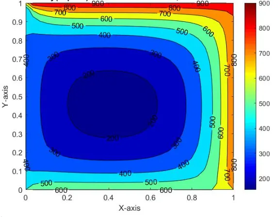
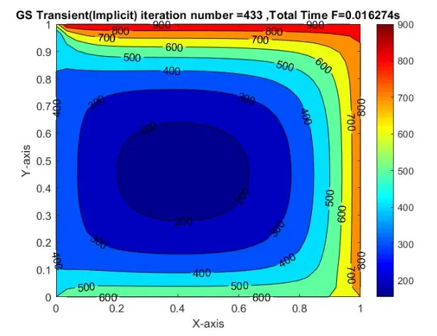
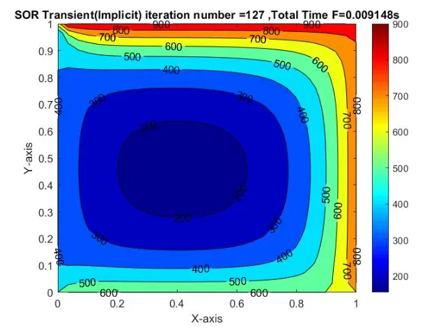
Transient Flow(Implicit) Output:-
Jacobi transient iteration(Implicit)
GS transient iteration(Implicit)
SOR transient iteration(Implicit)
RESULT:-
Comparing with the Different iteraions approaches and states, we can conclude the following things,The computational time and iteration required are SOR<GS
Between Explicit and Implicit results, the latter one does not depend greatly on Courant number for its stability and convergence, on the other hand in the Explicit approach information from a given cell or mesh element must propagate to its immediate neighbours, hence the low CFL number needs to be considered.