Week 8- Moving zones approach in Fluent

AIM :- 

1. What are the approaches by which you would model moving zones?
2. Which approach would you use to model unsteady phenomena?
3. Simulate rotary motion for the geometry given and Plot the Velocity Profile of Fluid Motion.

CONTENTS

Chapter 1 : - Overview of Moving Zones Approach and Approaches used to Model moving Zones

Chapter 2 : - Detailed Explaination of Moving Reference Frame (MRF) [Multiple Reference Frame].

Chapter 3 : - Approache Used for Unsteady Phenomenon

Chapter 4 : - Simulating Rotary motion for the given Geometry. And its detailed Explaination.

Appendix - Key take aways (Few Important Definitions).

Summary.

CHAPTER 1

OverView of Moving Zones Approach and Approaches used to Model moving Zones.

The solution of flows in moving reference frames requires the use of moving cell zones. This cell zone motion is interpreted as the motion of a reference frame to which the cell zone is attached. With this capability,
a wide variety of problems that involve moving parts can be set up and solved using FLUENT.

Overview of Moving Zones Approaches

• flow in a (single) rotating frame
• flow in multiple rotating and/or translating reference frames.

So in order to Model Moving Zones approaches Fluent has these set of Categories

(Example - In turbomachinery applications where rotor and stator blades are in close proximity (and hence rotor-stator interaction is important)).

1. The multiple reference frame (MRF) model
2. the mixing plane model
3. the sliding mesh model

[

Note - 

Both the MRF and mixing plane models assume that the flow field is steady, {Example - with the rotor-stator or impeller-baffle effects being accounted for by approximate means}. These can be acceptable models in cases where the rotor-stator interaction is weak or an approximate solution for the system is desired.

The sliding mesh model, on the other hand, assumes that the flow field is unsteady, and hence models the interaction with complete fidelity. This is the model of choice if rotor-stator interaction is strong and a more accurate simulation of the system is desired.

]

CHAPTER 2

Detailed Explaination of Moving Reference Frame (MRF) [Both - Single Reference Frame and Multiple Reference Frame] 

The Multiple Reference Frame 

FLUENT provides three approaches for modeling problems that involve both stationary and moving zones:

1. Multiple Reference Frame Model [MRF]

2. The mixing Plane Model

3. Sliding Mesh Model.

Now lets look into the details of The MRF model   (NOTE - Sliding Mesh model will be explained in the next Challenge , Here we deal only with MRF)

• The MRF is the simplest of all the three. multiple reference frame approach is clearly an approximation, it can provide a reasonable model of the time-averaged flow for many applications. For example, the MRF model can be used for a turbomachinery application in which rotor-stator interaction is relatively weak. In mixing tanks, since the impeller-baffle interactions are relatively weak, large-scale transient effects are not present and the MRF model can be used. In general, any problems where transients due to rotor-stator interaction are small are candidates for the MRF model.
• Another potential use of the MRF model is to compute a flow field that can be used as an initial condition for a transient sliding mesh calculation. This eliminates the need for a startup calculation.
• Strictly speaking, the use of multiple reference frames is meaningful only for steady flow.

The MRF formulation will depend on the velocity formulation being used.

1. Absolute Velocity Formulation
2. Relative Velocity Formulation

Relative Velocity Formulation

• In FLUENT’s implementation of the multiple reference frame feature, the calculation domain is divided into subdomains, each of which may be rotating/translating with respect to the laboratory (inertial) frame. The governing equations in each subdomain are written with respect to that subdomain’s reference frame.
• At the boundary between two subdomains, the diffusion and other terms in the governing equations in one subdomain require values for the velocities in the adjacent subdomain. FLUENT enforces the continuity of the absolute velocity, , to provide the correct neighbor values of velocity for the subdomain under consideration.
• When the relative velocity formulation is used, velocities in each subdomain are computed relative to the motion of the subdomain. Velocities and velocity gradients are converted from a moving reference frame to the absolute inertial frame.

Lets look into some basic Mathematical Steps involved in MRF

The position vector relative to the origin of the zone rotation axis is defined as

                                

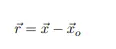
 = Position in absolute Cartesian

 = origin of the zone rotation axis

The relative velocity in the moving reference frame can be converted to the absolute (stationary) frame of reference using the following equation:

                         

 =  the velocity in the absolute inertial reference frame

 = the velocity in the relative noninertial reference frame

 = translational velocity of the noninertial reference frame.

Using this definition of absolute velocity, the gradient of the absolute velocity vector is given by

                   

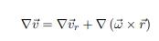
Absolute Velocity Formulation

When the absolute velocity formulation is used, the governing equations in each subdomain are written with respect to that subdomain’s reference frame, but the velocities are stored in the absolute frame. Therefore no special transformation is required at the interface between two subdomains.

So to summarize The MRF

1. Here Frame is Moving

2. Mesh Toplogy remains Same

3. No change in Control Volume (CV)

4. Steady Phenomenon

5. MRF Formulation depends on Velocity (Absolute and Relative Velocity) Formulation

6. Here Unsteadiness is not Important

CHAPTER 3

Approach Used for Unsteady Phenomenon

Moving Mesh Approach is used for Unsteady Phenomenon, and when we have a rotating wall that will change skewness of your element.

Used for Modelling Unsteady Phenomenon such as

• Vortex Induced Flows 
• Interaction of Vortex with bodies

Mesh is moving

Toplogy Changes with Time

Control Volume Changes with Time

Unsteady Phenomenon

If Unsteadiness is important

CHAPTER 4

PROBLEM SETUP AND SIMULATION OF THE ROTARY MOTION OF GIVEN GEOMETRY

step 1 :- Grid Generation. ---------   Import the given mesh file.

Two grid setup methods are available

1. If the boundary between two zones that are in different reference frames is conformal (i.e., the grid node locations are identical at the boundary where the two zones meet), you can simply create the grid as usual, with all cell zones contained in the same grid file. A different cell zone should exist for each portion of the domain that is modeled in a different reference frame. Use an interior zone for the boundary between reference frames.
2. If the boundary between two zones that are in different reference frames is non-conformal (i.e., the grid node locations are not identical at the boundary where the two zones meet), follow the non-conformal grid setup procedure.

Step 2 :- Probelm Setup

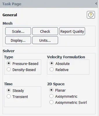
A. Select the Velocity Formulation to be used in the Solver panel: either Absolute or Relative

Choosing the relative and Absolute Velocity Formulation

• The absolute velocity formulation is preferred in applications where the flow in most of the domain is not rotating (e.g., a fan in a large room).
• The relative velocity formulation is appropriate when most of the fluid in the domain is rotating, as in the case of a large impeller in a mixing tank. 
• When one of the coupled solution algorithms is used, the absolute formulation is always used. the relative velocity formulation is not available in the coupled solvers.

B. Boundary Conditions

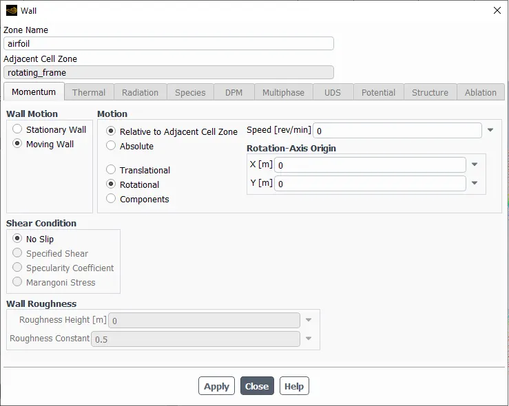
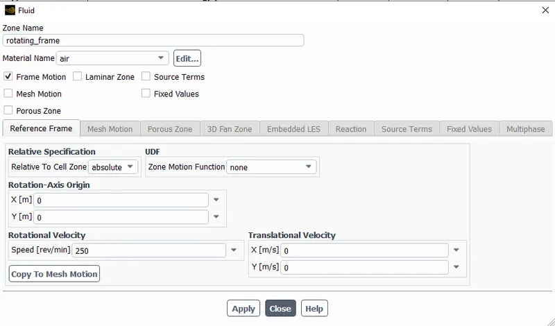
• For each cell zone in the domain, specify its translational velocity and/or its angular velocity (Ω) and the axis about which it rotates.
• If the zone is rotating, or if we plan to specify cylindrical velocity or flow-direction components at inlets to the zone, we will need to define the axis of rotation. In the Fluid panel or Solid panel, specify the Rotation-Axis Origin and Rotation-Axis Direction.
• Also in the Fluid or Solid panel, select Moving Reference Frame in the Motion Type drop-down list and then set the Speed under Rotational Velocity and/or the X, Y, and Z components
  of the Translational Velocity in the expanded portion of the panel.

C . Viscous Models

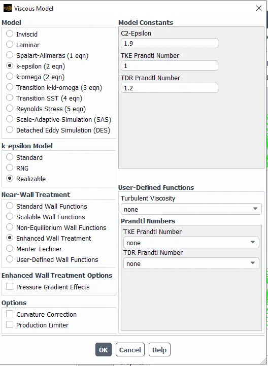
Until now, there is no one model that can predict all physical characteristics of turbulent flow. Various models are employed in the turbulent flow such as Direct Numerical Simulation (DNS), Reynolds Averaged Navier-Stroke (RANS), and Large Eddy Simulation (LES).  DNS has the best accuracy in turbulence solution. However, the required computational time and cost are relatively high.  The most common model used for solving Navier-Stokes equations is RANS.  The mathematical principle concept is based on the calculation method of the Navier–Stokes equation, which divides the flow into a fluctuating part and average part where the average equation is called the Reynolds decomposition.

Various turbulence models are used to solve the RANS equation

1. k-epsilon [RANS]
2. k-omega [RANS]
3. Transition Prediction Model [RANS]
4. Spalart Allamars Model [RANS]
5. Large Eddy Simulation Model [Non - RANS]
6. Detached-Eddy Simulation model [Non - RANS]

So the best one is choosen and Explained below.

k - ε Turbulence Models (RANS)

• The k - ε turbulence model series calculates the eddy viscosity by solving two parameters:
• firstly, the turbulent dissipation rate (ε) parameter;
• secondly, a turbulence kinetic energy (k) parameter.
• Standard k-ε was specified by Launder and Sharma, which is very popular and widely used;
• it (Standard k-epsilon) gives poor results for flow simulation that had a separation phenomenon such as separation at flow around the wind turbine at high wind speed.
• Another improvement and modification on standard k-ε have been done to attain the Renormalization Group (RNG) k - ε and Realizable k -ε turbulence models.
• Both models share the same transport equation as standard k-ε for turbulent kinetic energy (k) and dissipation rate (ε).
• However, the turbulent viscosity generation and calculation method mark the differences between these models.
• The renormalization group theory was used as a statistical method for solving the RNG k – ε turbulence model.
• The RNG k-ε turbulence has different modifications than standard k-ε, for example, considering the impact of rotation in eddy viscosity. The RNG k – ε is more accurate and better able to predict separations flows than standard k - ε.
• The realizable k - ε model is recommended for rotating bodies as the results could be improved when compared with standard k - ε for swirling flow problems under specific Reynolds number.

D. Solution Method

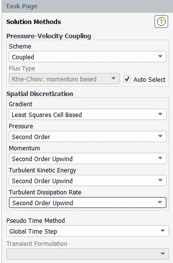
• The pressure-based solver allows you to solve your flow problem in either a segregated or coupled manner
• ANSYS FLUENT provides the option to choose among five pressure-velocity coupling algorithms: SIMPLE, SIMPLEC, PISO, Coupled, and (for unsteady flows using the non-iterative time advancement scheme (NITA)) Fractional Step (FSM).
• Note that SIMPLE, SIMPLEC, PISO, and Fractional Step use the pressure-based segregated algorithm, while Coupled uses the pressure-based coupled solver.
• The coupled scheme obtains a robust and efficient single phase implementation for steady-state flows, with superior performance compared to the segregated solution schemes.
• The coupled algorithm solves the momentum and pressure-based continuity equations together.
• The full implicit coupling is achieved through an implicit discretization of pressure gradient terms in the momentum equations, and an implicit discretization of the face mass flux, including the Rhie-Chow pressure dissipation terms (As you can see in below image).
• If you choose Coupled, you will have to specify the Courant number in the Solution Controls task page, which is set at 200 by default. You will also specify the Explicit Relaxation Factors for Momentum and Pressure, which are set at 0.75 by default.
• The second-order upwind scheme provides stability for supersonic flows and captures shocks better than the first-order upwind scheme.

E . Initialisation

• The Ansys Fluent Starts to Initialise at t = 0 condition
• Before starting your CFD simulation, you must provide ANSYS FLUENT with an initial "guess'' for the solution flow field. In many cases, you must take extra care to provide an initial solution that will allow the desired final solution to be attained.
• There are two methods for initializing the solution:
• Initialize the entire flow field (in all cells).
• Patch values or functions for selected flow variables in selected cell zones or "registers'' of cells. (Registers are created with the same functions that are used to mark cells for adaption.)

Here our problem involves moving reference frames, indicate whether the initial velocities are absolute velocities or velocities relative to the motion of each cell zone by selecting Absolute or Relative to Cell Zone under Reference Frame. (If no zone motion occurs in the problem, the two options are equivalent.) The default reference frame for velocity initialization in ANSYS FLUENT is relative. If the solution in most of our domain is rotating, using the relative option may be better than using the absolute option.

F. Results

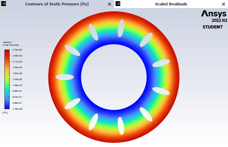
                                Figure 1 - Contours of Static Pressure

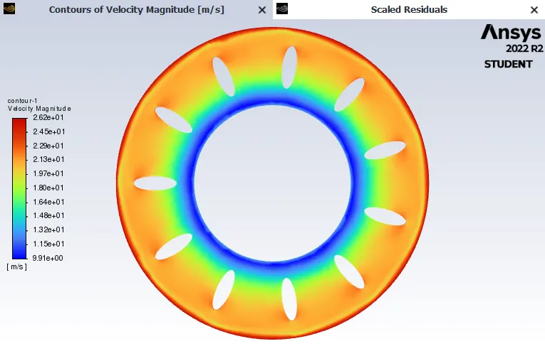
                       Figure 2 - Contours of Velocity Magnitude

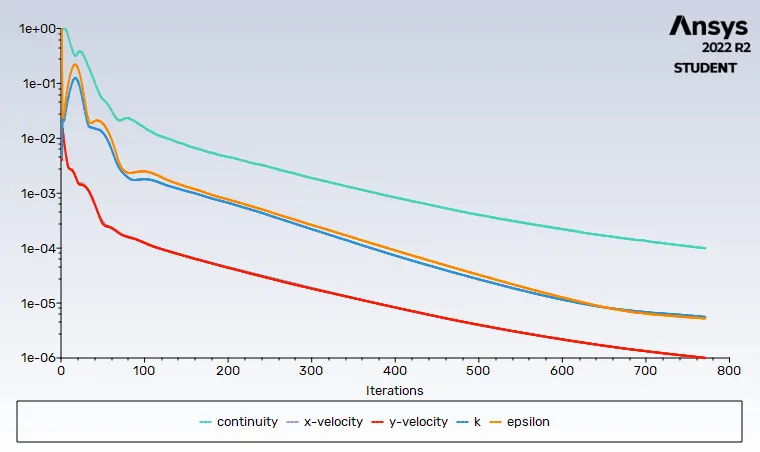
                                 Figure 3 - Residuals

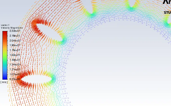
                      Figure 4 - Clear Image of Velocity Vectors

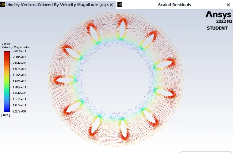
                           Figure 5 -  Velocity Vectors

Appendix - Key take aways (Few Important Definitions)

1. CFL Number

The Courant–Friedrichs–Lewy or CFL condition is a condition for the stability of unstable numerical methods that model convection or wave phenomena. As such, it plays an important role in CFD.

So,

the distance that any information travels during the timestep length within the mesh must be lower than the distance between mesh elements. In other words, information from a given cell or mesh element must propagate only to its immediate neighbors.

Where

Dt - Time step

Dx -  length between mesh elements.

a is the velocity magnitude.

for any explicit simple linear convection problem, the Courant number must be equal or smaller than 1, otherwise, the numerical viscosity would be negative:

2. How to Keep CFL Number less than 1?

The Courant number is a dimensionless value representing the time a particle stays in one cell of the mesh. It must be below 1 and should ideally be below 0.7. If the Courant number exceeds 1, the time step is too large to see the particle in one cell, it “skips” the cell. If it is smaller than 0.7, the particle stays in the cell for at least two time steps. 

These 2 images are enough to understand CFL Number.

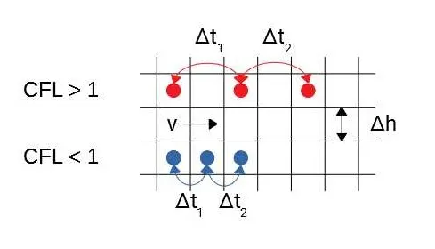
When the Courant number exceeds the value of 1, instabilities are amplified throughout the domain and may cause divergence of the simulation. Accordingly, to decrease the Courant number we can either:

• Decrease the time step Δt or
• Coarsen the mesh i.e. increase Δx

3. Absolute Velocity

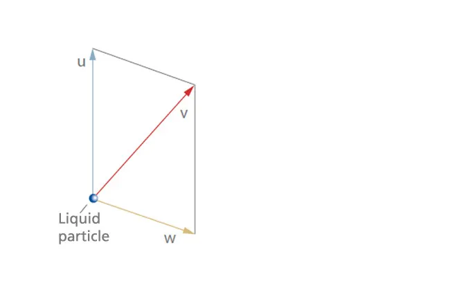
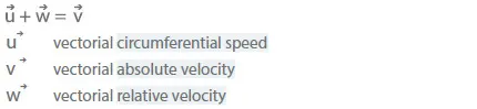
The concept of absolute velocity is mainly used in turbomachinery design and defines the velocity of a fluid particle in relation to the surrounding, stationary environment. Together with the relational Velocity and the circumferential Speed (u), it forms the velocity Triangle.

4. Relative Velocity

The concept of relative velocity (w) is used in turbomachinery design and defines the velocity of a fluid particle in relation to the rotating.

5. Velocity Triangle

The velocity triangle is the vectorial representation of kinematic movement. A vector is a directional magnitude. This relationship is illustrated in the velocity parallelogram of a liquid particle.

(Note - This is just the simplified explaination of Absolute velocity and relative velocity )

Flow angles in the velocity triangle

• Angle α between v and positive u direction ("absolute angle")
• Angle β between w and negative u direction ("relative angle")

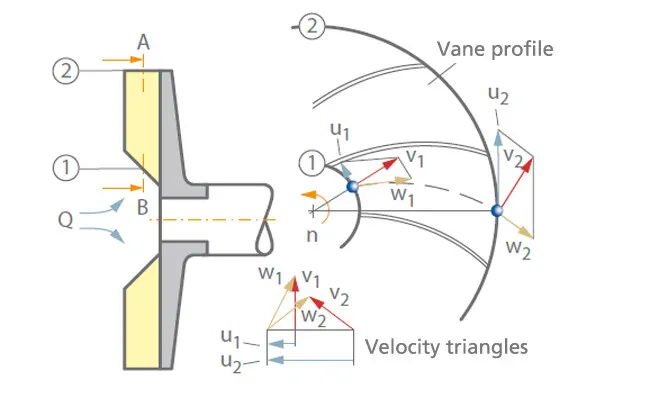
Figure 1 - Velocity triangle: Vane profile and velocity triangles for meridional section A-B through the radial impeller (longitudinal section through pump shaft)

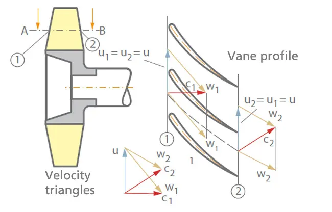
Figure 2 - Velocity triangle: Vane profile and velocity triangles for cylindrical section A-B through the axial impeller shown in meridional section.

6. Circumferential Speed

The circumferential speed (u) is the velocity of a point particle performing a circular motion. This can be a point particle of a rotating pump shaft or a rotating impeller.

Summary.

• Before starting a Problem try to understand what moving reference are we going to use.
• If we are using Multiple Refernce Frame - Then its important to know about the Absolute velocity and relative velocity formation.
• choose which elements are moving and set to moving conditions
• It is important to choose what elements are moving and giving the rotational or Translational and axis of origin based on the problem.
• It is also important to state the rotational speed on the moving reference frame
• CFL Number should be less than 1
• Choose the best solver type  - if it is pressure based choose any of the solution schemes, here we choosen Coupled approach as it solves pressure and momentum at a time
• Choose the Turbulence models, as it is the main factor for solving the fluid domain (As it comes with experience but some sort of knowledge is needed)
• Choosing the Boundary Conditions is a most vital role , if not stated properly the solution doesn't come.