Week 8- Moving zones approach in Fluent

There are two types of motion encountered in fluid flow, they are rectilinear and rotary.

There are two approaches to model rotary motion:

• Moving reference frame
• Moving mesh appraoch.

Moving refernce frame:

A Moving Reference Frame (MRF) is a relatively simple, robust, and efficient steady-state, Computational fluid dynamics modeling technique to simulate rotating machinery. For example, the rotors on a quadcopter can be modeled with MRFs.

The principal reason for employing a moving reference frame is to render a problem which is unsteady in the stationary (inertial) frame steady with respect to the moving rame. For a steadily rotating frame (i.e., the rotational speed is constant), it is possible
to transform the equations of fluid motion to the rotating frame such that steady-state solutions are possible. By default fluent permits the activation of a moving refernce frame with a steady rotational speed. If the rotational speed is not constant, the transformed equations will contain additional terms which are not inclkuded in fluent formulation. unsteady simulations can be studied in moving refernce frame with constant rotational speed.
wo approaches for multiple zones. It is a steady-state approximation in which individual cell zones can be assigned different rotational and/or translational speeds. The flow in each moving cell zone is solved using the moving reference frame equations If the zone is stationary ( ), the equations reduce to their stationary forms. At the interfaces between cell zones, a local reference frame transformation is performed to enable flow variables in one zone to be used to calculate fluxes at the boundary of the adjacent zone. The MRF interface formulation will be discussed in more detail in Section

It should be noted that the MRF approach does not account for the relative motion of a moving zone with respect to adjacent zones (which may be moving or stationary); the mesh remains fixed for the computation. This is analogous to freezing the motion of the moving part in a specific position and observing the instantaneous flowfield with the rotor in that position. Hence, the MRF is often referred to as the "frozen rotor approach."

While the MRF approach is clearly an approximation, it can provide a reasonable model of the flow for many applications. For example, the MRF model can be used for turbomachinery applications in which rotor-stator interaction is relatively weak, and the flow is relatively uncomplicated at the interface between the moving and stationary zones. In mixing tanks, for example, since the impeller-baffle interactions are relatively weak, large-scale transient effects are not present and the MRF model can be used.

Another potential use of the MRF model is to compute a flow field that can be used as an initial condition for a transient sliding mesh calculation. This eliminates the need for a startup calculation. The multiple reference frame model should not be used, however, if it is necessary to actually simulate the transients that may occur in strong rotor-stator interactions, the sliding mesh model alone should be used.

there are two types of moving reference frame approaches:

• Single moving reference frame.
• Multiple moving reference frame that uses a mixing plane approach.

contact region or the interface :

• this is the region existing in contact with the stationary plane or the moving plane.
• Section or region of intersection of the two frames.
• Circular type of interface
• The Navier stokes equation is the stationary frame and the moving frame is solved separately.
• Data is transferred from one frame to another through the interface

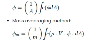
There are three methods of data transfer namely:

• Area averaging method
• 
• • Mixed approach

  In this approach the partial differntiation equations are solved. the momentum equation, wenergy equation, the continiuty equation is solved simulataneouisly.

  This approach gives the best result.

  • Moving mesh approach is used to model unstaedy flows. Generally flows with vortex induced and for the flows for inetraction of vortex with the bodies, moving mesh approach is used. In moving mesh methods, physical PDEs and a mesh equation derived from equidistribution of an error metrics (so-called the monitor function) are simultaneously solved and meshes are dynamically concentrated on steep regions
  • Simulation of the geometry:
  1. The meshed model is imported into ansys fluent.
  2. Preliminary mesh check is done.
  3. Under the general conditions, Pressure based solver is used. A steady state analysis is performed. Generally with moving refernce frame, steady state studies are conducted. . 2d planar analysis is doen.
  4. Under the models tab, turbiulence modelling is performed. both k omega SST and K epsilon model gives satisfactory results, but in this project, RNG K -epsilon model is used for analysis.
  5. The material for analysis is air.
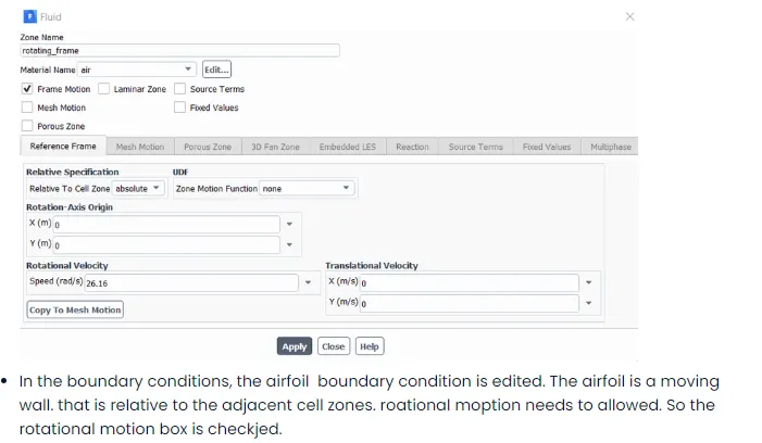
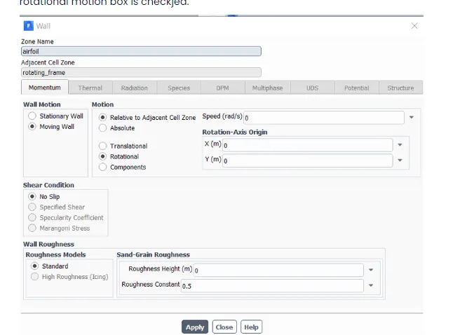
  6. In the cell zones, under the zones, rotating frame is enabled. Frame motion box is checked.

  In the roataion axis, the origin is set to (0,0) which is perfectly fine for this model.

  the angular velocity for this model is 250 rpm. there are two ways, either the value of the angular velocity is chamnged to radian per seconds or the units of the angu;lar velovcity is changed to rpm in fluent.

• 
• 

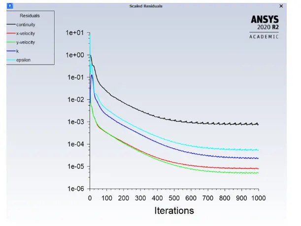
  This plot shows the solutions have converged.

  • The solution is run for 1000 iterartions.

  Velocity profile:

  

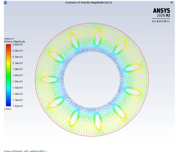
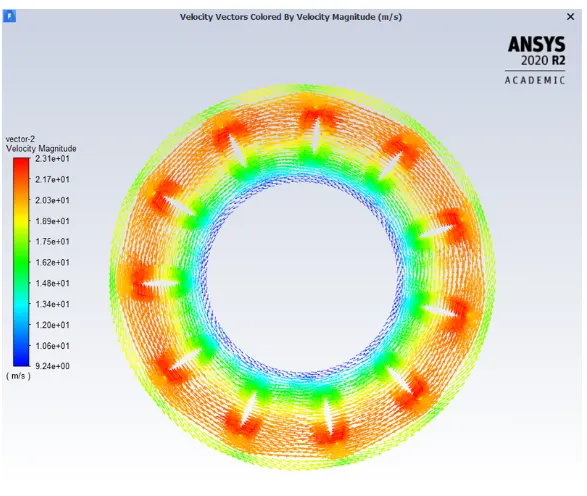
• Vevctors of velocity :

•