Week - 8 - Morphing

Objective :

To resize or morph the given object using the morphing method in ansa.

Theory :

What is a morphing?

Morphing is a special effect in motion pictures and animations that changes (or morphs) one image or shape into another through a seamless transition. Traditionally such a depiction would be achieved through dissolving techniques on film.

Mesh Morphing :

Mesh morphing consists of the adaption of a computational grid adopted for computer aided engineering (CAE). For instance, the solid or shell mesh of a structural part ready to be processed by an FEA solver, or the volume mesh complete with boundary conditions for a CFD solver, can take a new shape by just updating nodal positions. This means that the topology of the mesh (nodes count, cells count, connectivity) stays the same. Only the x,y,z coordinates of the nodes in the part of the model undergoing a shape modification are updated.

Mesh morphing can be used for different purposes: create shape parameters (i.e. change a length, an angle a thickness), move onto a new known shape (i.e. as manufactured, as designed by CAD), move onto a shape predicted by the CAE solution (automatic shape optimization with adjoint or BGM), and/or support multiphysics (move CFD mesh according to the evolution of the FEM-connected one, enable erosion/deposition).

Usually mesh morphing is faster than remeshing for a number of reasons: it avoids “remeshing noise” (having the same mesh adapted means the effect of a parameter is not confused with the effect of a new mesh structure), so variation effects can be assessed even with a coarser mesh. The CAE model can be updated on the background keeping all the original settings (boundary conditions). The update of nodal positions usually requires less computational efforts vs a full mesh regeneration. Creating shape parameters with mesh morphing is faster than creating a parametric CAD model.

Methods of morphing :

Morphing is accomplished by extracting the nodes of the baseline model surface, displacing these nodes (the actual morphing), and then remeshing the interior of the morphed geometry. The total displacement applied to the nodes is the linear combination of partial displacements, each one the result of parameterizing a factor of interest . We demonstrate three techniques for defining the partial displacements: a scaling-based (SB) technique to vary the thickness of the scleral shell; an analytic-based (AB)technique to change the diameter of the scleral canal; and a landmark-based (LB) technique to change the anterior-posterior position of the central lamina cribrosa (LC).

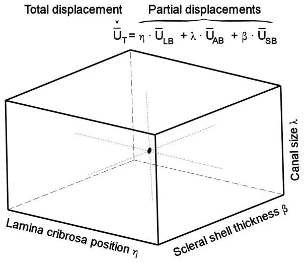
(The three-dimensional factor space. Each dimension corresponds to variations in a parameterized factor. The total deformation U_T applied to a node was the linear combination of the deformations defined for the parameterization of each factor: U_SB for the scaling-based morphing of scleral shell thickness, U_AB for the analytic-based morphing ofcanal size, and U_LB for the landmark-based morphing of lamina cribrosa position.)

Each partial displacement is the product of three components: a deformation field, a smoothing function, and a scaling constant. The deformation field defines the overall nature of the shape change. The smoothing function eliminates discontinuities and steep gradients in the deformation field that distort the surface mesh during morphing and hinder remeshing. The scaling constant sets the reference for the magnitude of the changes in shape and allows definition of the morphing in simple terms, such as double the thickness, or half the diameter. It is convenient to define partial displacements that are independent of each other. A simple way to achieve this is to base all the displacements on the baseline geometry. If the displacements are not independent, the scaling constants may become scaling functions, which are difficult to calibrate, complicating and reducing the generality of the analysis. In the end, there are two numbers setting the scale and sense of the morphing, the scaling portion of the definition of the partial displacement, and the linear coefficient of the parameterization. The techniques described below were implemented using C++ (Visual Studio v6.0, Microsoft, Redmond, WA), and Amira (vDev4.1.1, Visage Imaging, Carlsbad, CA). See the appendix for the equations and constants.

The baseline FE model geometry :

The techniques are demonstrated using a baseline specimen-specific FE model of the eye of a normal monkey reconstructed following a procedure we have described previously . The hex-based models of the lamina cribrosa and scleral shell used in our previous work were imported into Amira, converted to 4-node tetrahedral elements and refined twice. The triangulated surfaces were then extracted and smoothed to remove sharp angles. The baseline triangulated surface consisted of 28,398 nodes forming 57,254 triangles.

The model was translated and rotated so that the anterior lamina cribrosa surface centroid coincided with the origin (0,0,0), and the first, second and third moments of inertia coincided with the X, Z and -Y axes. This meant that the lamina cribrosa was roughly aligned with the XZ plane, the Y axis increased in the anterior direction. The origin was just anterior to the lamina cribrosa due to the natural curvature of its anterior surface.

Scaling-based (SB) deformations :

In SB morphing the deformation field, U_SB, is defined from a vector field implied by the geometry. In the example we parameterized the thickness of the scleral shell using a vector field, t, representing the scleral shell thickness at the nodes on the exterior scleral shell surface. The smoothing was a step function, f(r), where r was the distance from a node to the posterior lamina-sclera interface (the posterior insertion of the lamina cribrosa . This procedure was used to assign a deformation vector to the nodes on the exterior surface of the sclera. All other nodes were assigned a null deformation. Hence, deformations preserved the distribution of scleral thickness variations as well as the shapes of the interior scleral surface, the equator, the scleral canal and the lamina cribrosa. The scleral thickness vectors had a natural scale, the thickness of the baseline model, and therefore no further scaling of the deformation was necessary. When parameterized, the magnitude and sense of the change in scleral shell thickness was controlled by the parameter β, such that β=0.5 reduced the scleral shell thickness to half and β=−1 doubled the thickness.

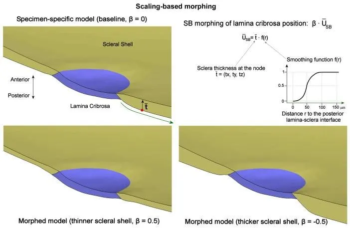
Scaling-based morphing technique illustrated by parameterizing the scleral shell thickness. The deformation U_SB is a scaling of the scleral thickness field t implied by the geometry multiplied by a smoothing function f(r), where r is the distance (green arrow) of a node (red dot) to the posterior lamina insertion into the sclera. Shown are cut-out views of three models: the baseline specimen-specific model (top left), and two models produced by the parameterization, one with a thinner scleral shell (bottom left), and another with a thicker scleral shell (bottom right).

Analytic-based (AB) deformations :

In AB morphing, the deformation field, U_AB, is defined by analytical functions . By combining relatively simple functions, it is possible to define complex deformations while maintaining control of the direction, sense and magnitude of the prescribed nodal displacements. In the example, to parameterize the size of the scleral canal we first computed a function g(a) for all the nodes. The vectors defined by g(a) were radial from the origin on the XZ plane, and had a zero component in the Y-direction. Smoothing was defined as a function of the elliptical distance to the origin, r, normalized using the vertical and horizontal radii of the scleral canal R_x and R_z. This function was chosen to prescribe an expansion which preserves canal wall shape and mesh quality. Unlike SB morphing methods, the scleral canal expansion deformation does not have an implied scale, so it was necessary to define one; in this case k₁=200 μm. When parameterized, the magnitude and sense of the changes in scleral canal expansion were controlled by the parameter λ such that λ=1 expanded the canal by 200 μm and λ=−1 shrunk the canal by 200 μm.

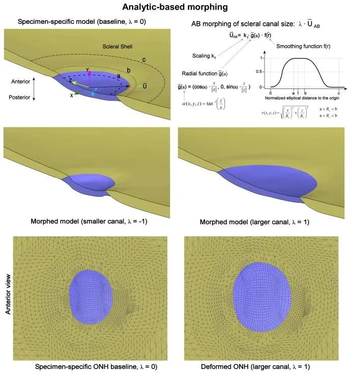
Analytic-based morphing technique illustrated by parameterizing the scleral canal size. The deformation U_AB (green arrow) is a flat (i.e. g_y = 0) vector in the radial direction g(α) multiplied by a smoothing function f(r), where r is the normalized elliptical distance to the origin. The magnitude of the smoothing function varies from 0 at the origin, to 1 between a and b (dashed and dotted lines, respectively on the top left plot), to 0 again at r=c (dash-dotted line on the top left plot). The constants a, b were chosen to include the canal wall. Shown are three models: the baseline specimen-specific model (top left), and two models produced by the parameterization, one with a smaller scleral canal (middle left), another with a larger scleral canal (middle right). Also shown are anterior views of the models with the elements outlined to illustrate how the morphing has changed the size of the canal, but it has not distorted the mesh substantially (bottom row).

Landmark-based (LB) deformations :

In LB morphing, the deformation field, U_LB, is defined as the product of a warping field h(r), a smoothing function f(r), and a scaling constant k₂ . The warping field is defined through corresponding sets of “source” and “target” landmarks located in space. The classical Bookstein thin-plate spline method is then used to compute a 3D warping of space matching the source to the target landmarks . In the example, we used nine landmarks on each of the anterior and posterior surfaces of the lamina cribrosa to parameterize the anterior-posterior position of the lamina cribrosa. The target landmarks were placed using a combination of manual displacements and scaling . The method produced a smooth deformation field h(r), which was restricted, also smoothly, by f(r), to deform only the portions of the structure intended. We used separate smoothing functions for the anterior and posterior surfaces of the lamina to allow more precise control of the smoothing at the edges and limit the deformations to the lamina cribrosa. The scaling constant k₂=0.66 was chosen so that the negative of the displacement produced by the deformation field output of the Bookstein method produced a flat lamina cribrosa (i.e. an anterior lamina cribrosa with zero average depth relative to its periphery, left panel, middle row). When parameterized, the magnitude of the changes in lamina cribrosa position were controlled by the parameter η such that η<0 produced a shallower lamina (a flat lamina when η=−1) and η>0 produced a deeper lamina.

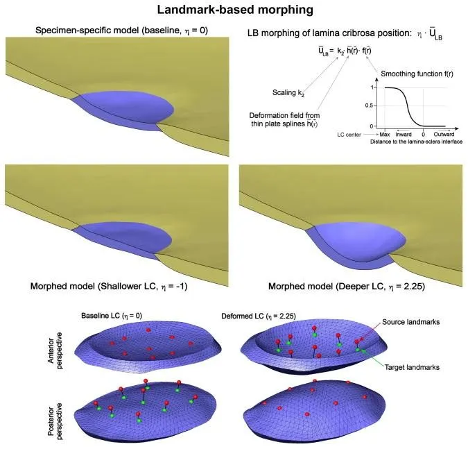
Landmark-based morphing technique illustrated by parameterizing the lamina cribrosa anterior-posterior position. The deformation U_LB is the product of a warping field h(r), a scaling constant k₂, and a smoothing function f(r). The warping field was defined using a Bookstein thin-plates spline method based on placing “source” (red dots) and corresponding “target” (green dots) landmarks. The smoothing is a function of the distance to the lamina-sclera interface, with magnitude zero outside the lamina, and increasing gradually from 0 at the lamina-sclera interface to 1 at the lamina center. Three models are shown in the top two rows: the baseline specimen-specific model (top left), and two models produced by the parameterization, one with a shallower (flat) lamina cribrosa (middle left), another with a deeper lamina cribrosa (middle right). The bottom row shows the whole lamina cribrosa of the baseline (left side) and deeper lamina (right side) models, from the anterior or posterior perspectives. We have outlined the elements to illustrate how the deformation has not distorted the element shapes substantially. Note that in the anterior perspective we only show landmarks that determine the warping of the anterior lamina surface, and in the posterior perspective we only show landmarks that determine the warping of the posterior lamina surface.

Methods used in ANSA :

Domain (Box) Morphing :

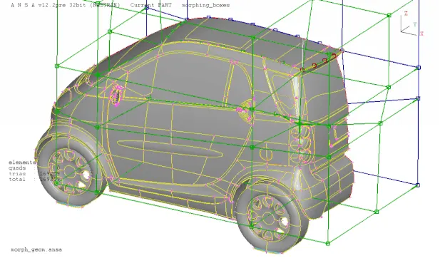
Domain or Box Morphing is preformed via boxes that are created around a particular part or assembly that the user intends to morph. The movement of the Morphing boxes control points defines the morphing operations on the entities inside the Morph box. This type of Morphing can be applied to both FE and Geometry based models.

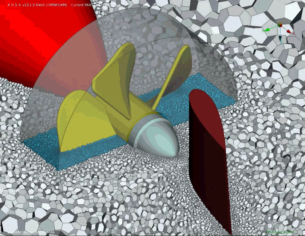
Direct Morphing

ANSA’s Direct morphing features gives the user the ability to efficiently modify a part locally without having to create Morphing boxes. This method is extremely useful in creating local modifications on single parts. Creation of depressions, surface fitting certain FE part features to new target geometry, moving selected features along the contour of a surface and also the ability to freeze (rigid) elements during the morphing process are some of the direct morphing abilities.

Parametric Morphing :

The desired morphing actions can be saved as parameters which can be accessed in batch mode. Users can enforce desired shape changes by changing numerical input value for the appropriate parameter. This method of morphing is highly utilized for coupling of the morphing operations to an external optimizer. The scripting capability can be used in conjunction with ANSA’s parametric morphing functionality to deliver faster DOE models.

Geometry Morphing :

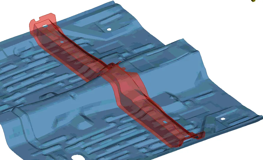
ANSA brings to the CAE world its ‘one – of – a kind’ tool for CAD geometry morphing. This pioneering concept allows the user to utilize the inventory of all the familiar FE morphing functions to perform equivalent operations in a CAD environment on geometric entities.

Procedure :

Step 1: Import the model to the ansa and after importing apply topo the model to get the complete model.

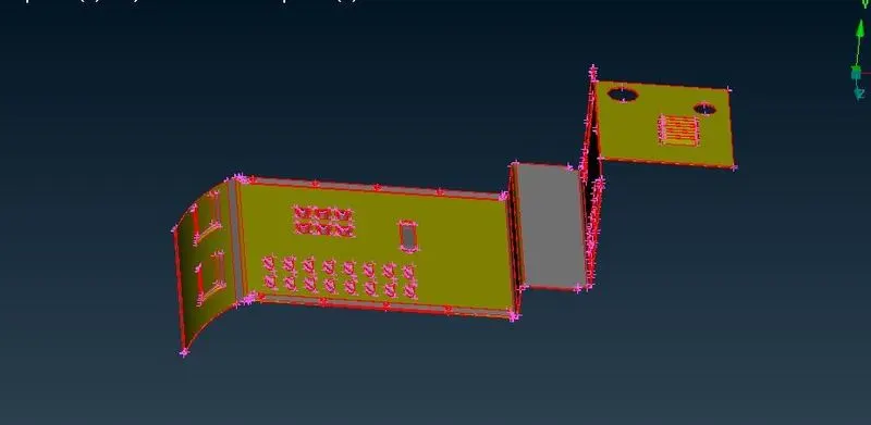
Step 2: After that go to the checks manager and select geomentry option and execute it and clear the errors.

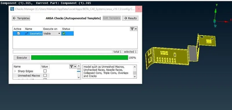
Step 3: Now we have to perform a morphing on the geomentry in order to do that go to morph deck.

Step 4: To perform morphing on the geomentry first we needto create a box like volume where it has the node points or points which will help to move the respected geomentry. So, go to the new select the ortho to create the box.

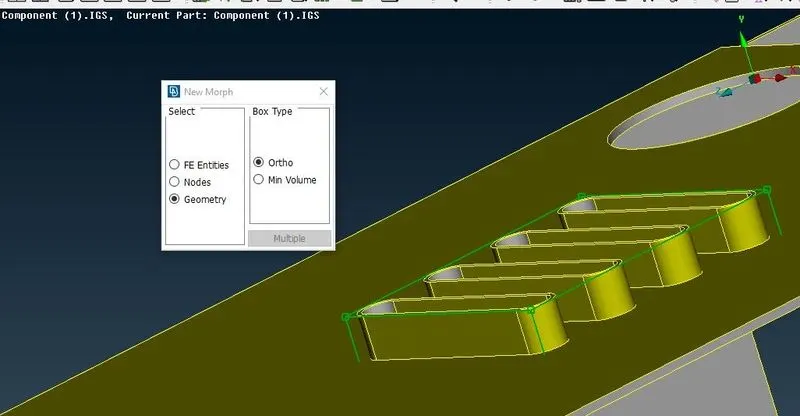
Step 5: Now we have created a morph box, to morph the geomentry we need to use move option and with this option we can select the nodes of the morph box and we pick the direction which we have to move.

Step 6: Thus we can perform a morph on given geomentry, here we have performed a basic morphing.

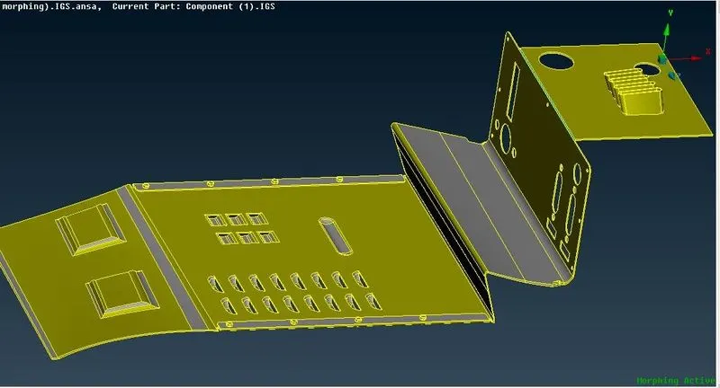
Results :

Thus we have learnt how to perform a morphing for basic model in ansa and also learnt methods in ANSA and how it works.