Week - 8 Mass Scaling
AIM:
The objective of the report is to perform mass scaling stability analysis for explicit solver and validate the results with implicit analysis.
THEORY:
Mass Scaling -
In explicit solver, the time step is decided by using Courant-Friedrichs-Levy criterion. It states that the time step must be smaller than a elastic wave to propagate from one side of the element to the other side of the element.
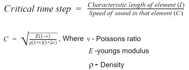
From CFL criteria, time step(dt) ≤ Critical time step
The time step(dt) is calculated for every element and minimum of all dt is selected as time step. So, the properties of the elements decides the time step size.
Suppose in a cad model, if some elements have low characteristic length which results large computational time which is not feasible. So, mass scaling is applied to those elements. In mass scaling, the density of the elements is increased so that the time step is increased which reduces the overall computational time.
KEYWORD IN LS DYNA -
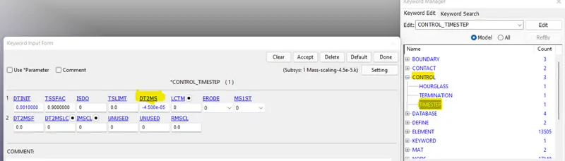
In LS-DYNA, DT2MS parameter in *CONTROL_TIMESTEP card is used to add non-physical mass to the element.
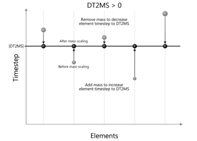
DT2MS > 0, the non-physical mass is added and removed to adjust the time step to required value.
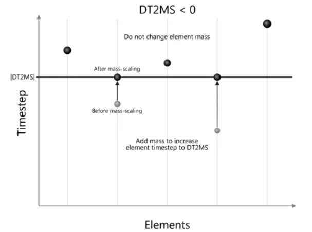
DT2MS < 0, the non-physical mass is only added to adjust the time step to required value as shown in the fig.
PROCEDURE:
In this report, the model is simulated by using both explicit and implicit solvers and results are validated.
1) Explicit solver -
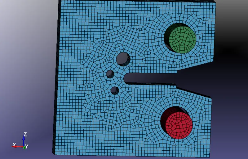
Import the model in LS-DYNA as shown in the fig.
It is advised to keep mass added percentage < 8%, so that there is no too much variation in results.
As discussed above, DT2MS parameter is responsible for mass scaling.
TSSFAC parameter is the scaling factor of the time step, it only affects the overall computational time. It does not affects mass scaling. Genearally, it is advised to keep 0.6 ≤ TSSFAC ≤ 0.9
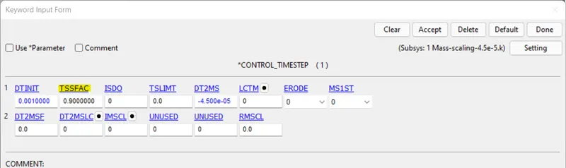
By trial and error method, we are simulating the the model for different values of dt2ms and tsfac. The termination time is set as 600sec.

The table-1 and table-2 shows the percentage added mass and overall computational time for time scaling factor of 0.9 and 0.6.
| S.NO | TSSFAC | DT2MS | Percentage mass added | COMPUTATIONAL TIME |
| 1 | 0.9 | -4.5e-5 | 0 % | 9hr:38min |
| 2 | 0.9 | -5.5e-5 | 1.0034e-2 % | 8hr:14min |
| 3 | 0.9 | -7.5e-5 | 0.3728 % | 6hr:09min |
| 4 | 0.9 | -9.5e-5 | 4.313 % | 4hr:52min |
| 5 | 0.9 | -1e-4 | 6.423 % | 4hr:40min |
| 6 | 0.9 | -1.5e-4 | 1.143e2 % | 3hr:13min |
| 7 | 0.9 | -4.5e-4 | 1.7419e3 % | 1hr:3min |
TABLE 1 - Time scaling factor 0.9
| S.NO | TSSFAC | DT2MS | Percentage mass added | COMPUTATIONAL TIME |
| 1 | 0.6 | -4.5e-5 | 0 % | 15hr:38min |
| 2 | 0.6 | -5.5e-5 | 1.0034e-2 % | 14hr:18min |
| 3 | 0.6 | -7.5e-5 | 0.3728 % | 9hr:49min |
| 4 | 0.6 | -9.5e-5 | 4.313 % | 8hr:12min |
| 5 | 0.6 | -1e-4 | 6.423 % | 7hr:54min |
| 6 | 0.6 | -1.5e-4 | 1.143e2 % | 5hr:40min |
TABLE 2 - Time scaling factor 0.6
From table 1 and table 2, it is observed that -
- As DT2MS increases, percentage added mass also increases and overall computational time decreases. For dt2ms = -1.5e-4, the percentage added mass is 114.3% which is not feasible, it leads to false results.
- The TSSFAC only affects the computational time, it does not affects the percentage mass added. If TSSFAC is reduced, then the step time size also decreases, which in turn increases the overall computational time.
CONTOUR PLOTS -
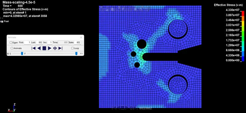
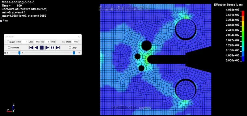
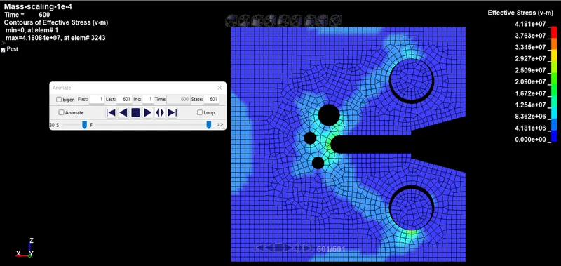
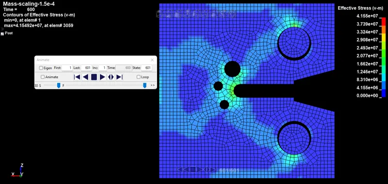
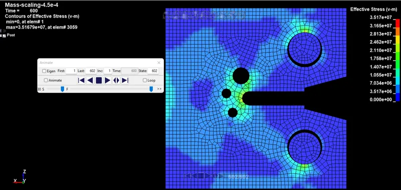
Inorder to do analysis for mass scaling, it is advised to compare force-related plots like stress, energy etc. As, in mass scaling the mass of elements gets altered which affects the stress and energy plots. The displacement plots are not affected due to mass scaling. So, effective stress plots for tssfac = 0.9 is compared for different dt2ms values.
The following fig shows the contour plots of effective stress for the model for tssfac = 0.9
| S.NO | DT2MS | Maximum effective stress | Percentage mass added | absolute Percentage error |
| 1 | -4.5e-5 | 4.329e7 | 0 % | 0 % |
| 2 | -5.5e-5 | 4.068e7 | 1.0034e-2 % | 6.029 % |
| 3 | -1e-4 | 4.180e7 | 6.423 % | 3.44 % |
| 4 | -4.5e-4 | 3.516e7 | 1.741e3 % | 18.78 % |
TABLE 3 - Maximum effective stress for different dt2ms
From the table 3, for dt2ms = -4.5e-5, the percentage mass added is 0%. So, it is taken as reference value. It is observed that for dt2ms = -4.5e-5, the % mass added is 1.74e3%, the % error in maximum effective stress is 18.78%. So, it is not feasible to use dt2ms = -4.5e4 as it results in false solution.
PLOTS FOR DIFFERENT TSSFAC -
From table 1 and table 2, it is observed that time scaling factor doesn't affect the percentage increase in mass.
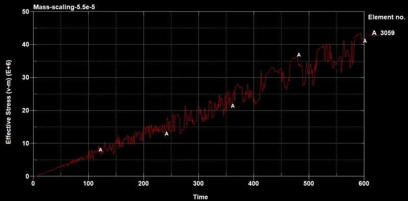
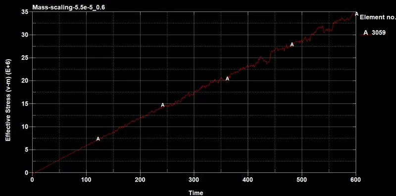
For tssfac = 0.6, the dt is less compared to tssfac = 0.9. It is known that the accuracy of solution increases for low dt value. So, in the following fig, it is observed more zig zag pattern for tssfac = 0.9 compared to tssfac = 0.6.
So, tssfac = 0.6 produces accurate results compared to tssfac = 0.9.
2) Implicit solver -
Since, in implicit solver, the solution is unconditionally stable, the time step size don't have any crucial role as like explicit solver.
In implicit analysis, the accuracy depends on the tolerance limit
Keywords used in implicit solver -
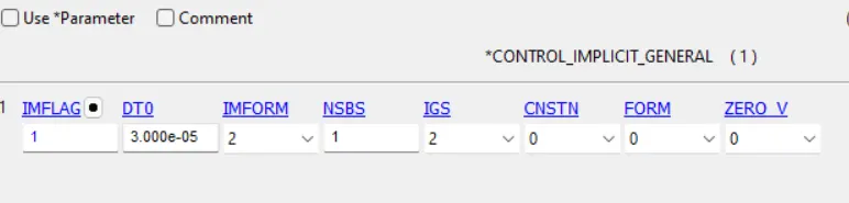
1) *CONTROL_IMPLICIT_GENERAL - It is the essential keyword used to implicit analysis. IMFLAG = 1, activates implicit solver.
2) *CONTROL_IMPLICIT_AUTO - It is used to adjust the time step size to achieve convergence.

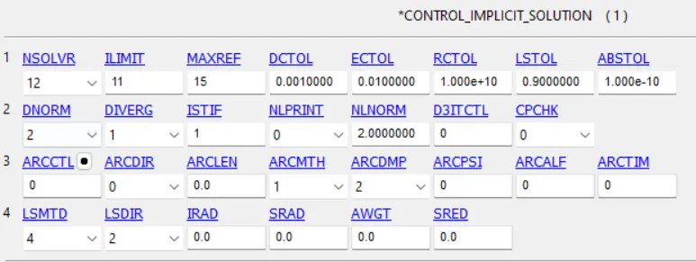
3) *CONTROL_IMPLICIT_SOLUTION - The tolerance limits, maximum reformations are inputed in this keyword. Also, non-linear solver
4) *CONTROL_IMPLICIT_SOLVER - This keyword is to give input about linear solver.
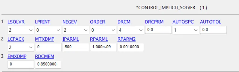
In the above implicit cards, the same time conditions are applied to implicit solver as like in explicit solver case like DT0 = 3e-5, DTMIN = 3e-5, DTMAX = 1e-4.
The termination time is 600 sec.
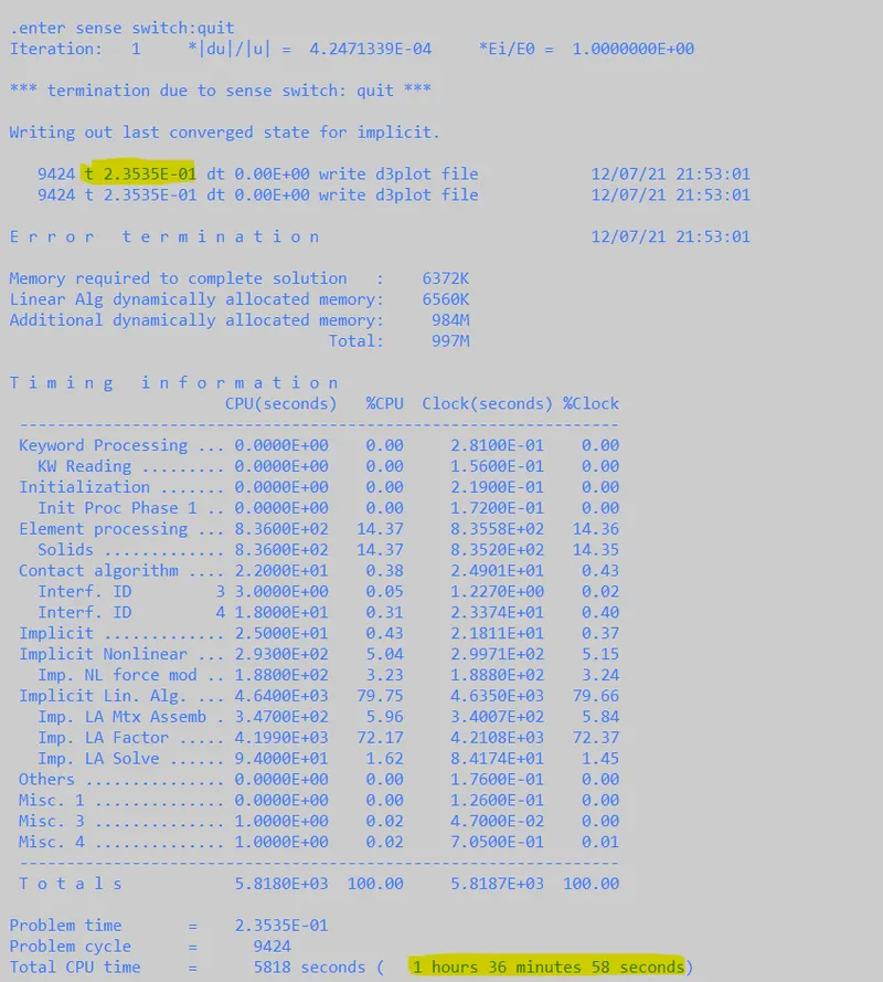
By running the implicit solver by the above conditions, inorder to solve for t = 0.235 sec out of 600sec, it takes nearly 1hr36min. So, to solve total 600 sec, the computational time is approximated nearly as 4126 hr 14 min, which is infeasible.
So, in the above implicit cards, the time conditions are modified a little bit and the analysis is done. DT0 is changed to 1.
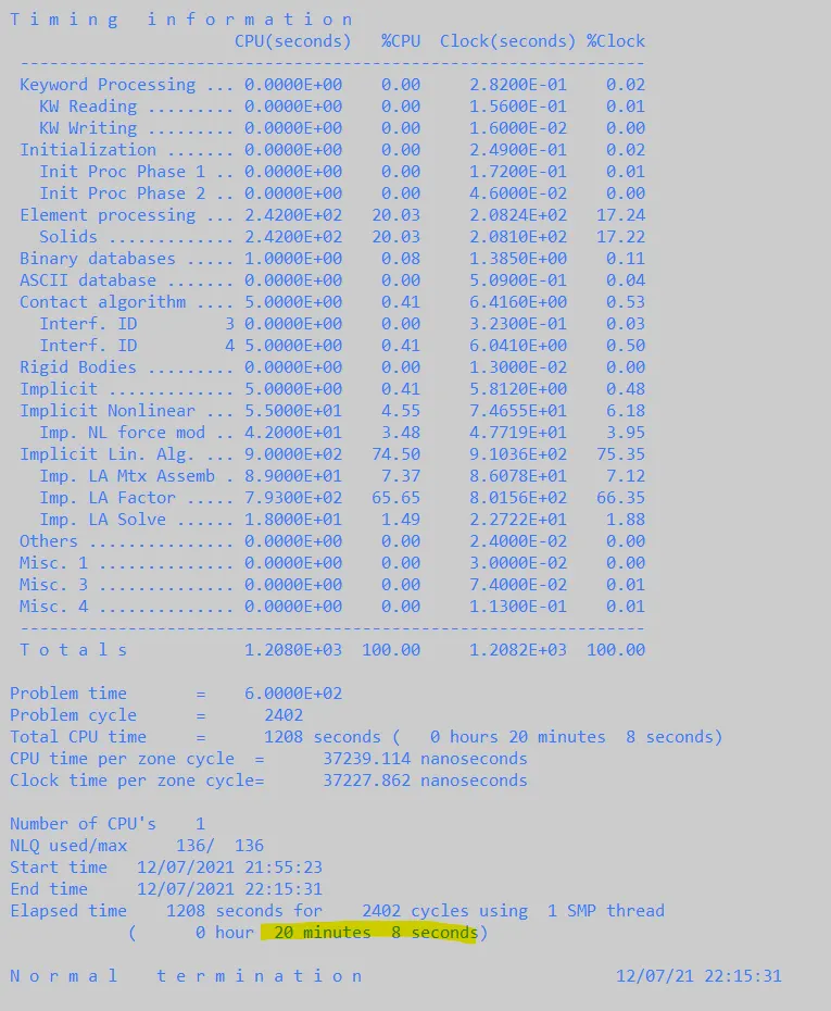
The computational time to solve the model with above conditions is 20min 8sec.
IMPLICIT V/S EXPLICIT SOLVER -
| Solver | Time step | Computational time |
| Explicit | 4.5e-5 | 9hr 38min |
| Implicit | 3e-5 | 4126hr 14min |
From the above table, for dt = 4.5e-5, the explicit solver computational time is 9hr 38 min and for dt = 3e-5, the implicit solver computational time is 4126hr 14min. It is observed that computational time for Implicit solver is very high when compared for explicit solver so same input conditions.
CONCLUSION:
It is concluded that in mass scaling, as the percentage mass added increases the computational time decreases and it is advised to limit percentage mass added to less than 8%. The computational cost for Implicit solver is high compared to Explicit solver.